Gelöste Aufgaben/JUMP/Car-Body

← Back to Start

Scope

Car-Body

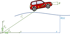
In common simulation applications - especially for full-size commercial cars - the pitch-angle of the car is assumed to be small to allow for a linearization of geometry and most parts of the equations of motion. We drop this limitation so we can do more fancy stuff with our model - like climbing steep roads or jumping across ditches.

Block Diagram.

We employ a spatial x-y coordinate system, x in horizontal, y in vertical, upwards direction. And we’ll briefly employ the z-axis as rotation direction - which is towards you following the “right-hand-rule“ for coordinate systems.

Structure

The driver controls the car's motion via the position of the "gas"-pedal, which is being translated into a torque M_W at the wheel.

This toque will change velocities and thus the position of the car. These state-variables will then create - via info - a feedback to the driver.

We’ll need to invest significant efforts in describing the kinematics of the car-motion and to derive its equations of body-motion since we do not want to limit our study on small pitch-angles of the car. Key accessory will be vectors, which map locations like the center of mass:

${\overrightarrow{r}}_C(t)$.

This vector has - in 2D - two coordinates $u_1(t),u_2(t)$, measured in the inertial x-y frame:

${\overrightarrow{r}}_C(t)={\overrightarrow{\underset{\_}{e}}}_0\cdot \left(\begin{array}{c}{u}_1\\ u_2\end{array}\right)$ with ${\overrightarrow{\underset{\_}{e}}}_0=({\overrightarrow{e}}_x,{\overrightarrow{e}}_y)$.

representing the unit vectors spanning the x-y space. If we refer to a specific frame, we may drop the vector-notation $(\overrightarrow{.})$ and refer to the column-matrix of coordinates $(\underset{\_}{.})$ only, so

${\underset{\_}{r}}_C=\left(\begin{array}{c}{u}_1\\ u_2\end{array}\right)$.

We’ll also employ coordinate transformations using Euler-rotations.

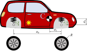
The car with front-wheel drive consists of the car-body with center of mass “C“, the front wheels “A“ and the rear wheel “B“. Masses of car-body and wheel-sets are M and m respectively.The geometry of the car is described by

• a₀: the wheel base;
• a₁: longitudinal distance between center of mass and front-wheel-hub;
• a₂ = a₀ - a₁ and
• a₃: vertical distance between center of mass and front-wheel-hub (relaxed springs).

tmp

Body

We use five coordinates to describe the motion of the car:

• $u_1(t),u_2(t),\phi (t)$ for the location of the center of mass of the car-body and its pitch-angle
  ,
• $u_3,u_4$ for the "vertical" motion of the wheel hubs relative to the car-body - which is synonym to the compression of the springs
  
  and
• $\psi (t)$ as the rotation angle of the front-wheel - we'll not account for the rotation of the rear-wheel.

So the center of mass of the car-body is

${\overrightarrow{r}}_M={\overrightarrow{\underset{\_}{e}}}_0\cdot \left(\begin{array}{c}{u}_1(t)\\ u_2(t)\end{array}\right)$,

the coordinate system of the car is

${\overrightarrow{\underset{\_}{e}}}_C={\overrightarrow{\underset{\_}{e}}}_0\cdot \underset{\_}{\underset{\_}{D}}(\phi (t))$

where

$\underset{\_}{\underset{\_}{D}}(\phi )=\left(\begin{array}{rr}\cos (\phi )& -\sin (\phi )\\ +\sin (\phi )& \cos (\phi )\\ \end{array}\right)$.

So the location of the front-wheel “A“ is

${\overrightarrow{r}}_A={\overrightarrow{r}}_M+{\overrightarrow{r}}_{MA}$

or

${\underset{\_}{r}}_A={\underset{\_}{r}}_M+\underset{\_}{\underset{\_}{D}}(\phi (t))\cdot \left(\begin{array}{c}{a}_1\\ -a_3+u_3(t)\end{array}\right)$.

Likewise, the location of the rear-wheel “B“ is

${\underset{\_}{r}}_B={\underset{\_}{r}}_M+\underset{\_}{\underset{\_}{D}}(\phi (t))\cdot \left(\begin{array}{c}-a_2\\ -a_3+u_4(t)\end{array}\right)$

and in the following, we’ll be using the abbreviations

$\left(\begin{array}{c}{U}_3\\ U_4\end{array}\right)=:{\underset{\_}{r}}_A$

and

$\left(\begin{array}{c}{U}_5\\ U_6\end{array}\right)=:{\underset{\_}{r}}_B$.

tmp

Track

Tack specification

We describe the road by road-sections, which we call tracks. We start by defining each track as a line-segment, i.e. a first-order polynomial. The road is thus defined by pairs of track-endpoints, i.e. (x_i, y_i).

The track-polynomials are

$\begin{array}{ll}{t}_i(x)& =y_i\cdot {\tilde{x}}_i+y_{i-1}\cdot (1-{\tilde{x}}_i)\text{ for }{\tilde{x}}_i=\frac{x-x_{i-1}}{x_i-x_{i-1}}\\ & =T_{i,1}\cdot x+T_{i,0}\end{array}$.

During the numerical integration of the initial-value-problem - when the car runs along the track - the solver needs to cope with the transition between two straight lines - which is numerically more efficient if we convert the road in a continuously differentiable function.

Rounding the edges.

For this purpose, we define transition polynomials p_i of second degree - parabolas - as

$p_i(x)=\sum _{j=0}^2{P}_{i,j}\cdot x^j$

which connect two neighboring tracks.

The boundary conditions for the parabolas (red) and the neighboring lines (blue) yield

$\begin{array}{ll}{t}_i(x_i-\mathrm{\Delta }{x}_i)& =p_i(x_i-\mathrm{\Delta }{x}_i),\\ {\frac{d{t}_i}{d{x}_i}|}_{x_i-\mathrm{\Delta }{x}_i}& ={\frac{d{p}_i}{d{x}_i}|}_{x_i-\mathrm{\Delta }{x}_i},\\ t_{i+1}(x_i+\mathrm{\Delta }{x}_i)& =p_i(x_i+\mathrm{\Delta }{x}_i),\\ {\frac{d{t}_{i+1}}{d{x}_{i+1}}|}_{x_i+\mathrm{\Delta }{x}_i}& ={\frac{d{p}_i}{d{x}_i}|}_{x_i+\mathrm{\Delta }{x}_i}.\end{array}$

And though we have four boundary conditions, they allow for a solution with three unknown polynomial coefficients P_i if Δx_i is identical left and right from x_i - which we have already implied.

$\begin{array}{ll}{b}_3& =0,\\ b_2& =\frac{a_{2,1}-a_{1,1}}{4\mathrm{\Delta }{{x}}_{{i}}},\\ b_1& =\frac{(a_{2,1}+a_{1,1})\mathrm{\Delta }{{x}}_{{i}}-x_i{a}_{2,1}+x_i{a}_{1,1}}{2\mathrm{\Delta }{{x}}_{{i}}},\\ b_0& =\frac{(a_{2,1}-a_{1,1}){\mathrm{\Delta }{{x}}_{{i}}}^2+(-2x_i{a}_{2,1}-2x_1{a}_{1,1}+4y_i)\mathrm{\Delta }{{x}}_{{i}}+x_i^2{a}_{2,1}-x_i^2{a}_{1,1}}{4\mathrm{\Delta }{{x}}_{{i}}}\end{array}$

and

$\begin{array}{ll}{a}_{1,0}& =y_i-x_i{a}_{1,1},\\ a_{1,1}& =\frac{y_{i-1}-y_i}{x_{i-1}-x_i},\\ a_{2,0}& =y_i-x_i{a}_{2,1},\\ a_{2,1}& =\frac{y_i-y_{i+1}}{x_i-x_{i+1}}\end{array}$

But instead of employing the above, we solve the linear systems of equations for the coefficients numerically.

Now each polynomial creates new endpoints x_i - Δx_i and x_i + Δx_i which substitute for the initial x_i-point. The tracks are represented by a succession of lines and parabolas.

Next we need to find the contact point between wheel and road!

/*******************************************************/
/* MAXIMA script                                       */
/* version: wxMaxima 16.04.2                           */
/* author: Andreas Baumgart                            */
/* last updated: 2021-02-08                            */
/* ref: Modelling and Simulation (TUAS)                */
/* description: Rounding between straight line-segments*/
/*******************************************************/

/*******************************************************/
/* declarations                                        */
/*******************************************************/
declare("Δ",alphabetic);

params: [x[0] = 0, x[1] = 10, x[2]=15,
         y[0] = 0, y[1] =  1, y[2]=-1,
	 eps = 0.2];

/*******************************************************/
/* polynomials                                         */
/*******************************************************/
/* polynomial coefficiets of two consecutive straigt lines */
P : [[a[1,1],a[1,0]],[a[2,1],a[2,0]]];
/* polynomials of cubic and two consecutive linear polynomials */
p : [a[1,1]*x+a[1,0],
     b[3]*x^3+b[2]*x^2+b[1]*x+b[0],
     a[2,1]*x+a[2,0]];

/* compute polynomial coefficients from (x[i]/y[i])-points*/
linear : solve([subst([x=x[0]],p[1]) = y[0],
                subst([x=x[1]],p[1]) = y[1],
		subst([x=x[1]],p[3]) = y[1],
		subst([x=x[2]],p[3]) = y[2]], [a[1,0],a[1,1],a[2,0],a[2,1]])[1];
/* equations to continuously fit cubic function to lines */
equs : [subst([x=x[1]-Δx], p[1]) = subst([x=x[1]-Δx], p[2]),
        subst([x=x[1]+Δx], p[3]) = subst([x=x[1]+Δx], p[2]),
	subst([x=x[1]-Δx], diff(p[1],x)) = subst([x=x[1]-Δx], diff(p[2],x)),
	subst([x=x[1]+Δx], diff(p[3],x)) = subst([x=x[1]+Δx], diff(p[2],x))];
/* unknowns */
Q : [b[3],b[2],b[1],b[0]];

/* solve for unknowns */
sol : ratsimp(subst(linear,solve(equs,Q)[1]));

/* solve linear system of equations for unknown coefficients */
ACM : augcoefmatrix(equs,Q);
print(submatrix(ACM,5)," * ",transpose(Q)," = ",col(ACM,5))$


/* or - more simple when doing it numerically  .... */

/* coefficients of straigt line polynomials */
s : makelist(a[i,1] = (y[i-1]-y[i])/(x[i-1]-x[i]),i,1,2);

P : [[a[1,1],a[1,0]],[a[2,1],a[2,0]]];
p : [a[1,1]*x+a[1,0],
     b[3]*x^3+b[2]*x^2+b[1]*x+b[0],
     a[2,1]*x+a[2,0]];

linear : solve([subst([x=x[1]],p[1]) = y[1],
		subst([x=x[1]],p[3]) = y[1]], [a[1,0],a[2,0]])[1];

equs : [subst([x=x[1]-Δx], p[1]) = subst([x=x[1]-Δx], p[2]),
        subst([x=x[1]+Δx], p[3]) = subst([x=x[1]+Δx], p[2]),
	subst([x=x[1]-Δx], diff(p[1],x)) = subst([x=x[1]-Δx], diff(p[2],x)),
	subst([x=x[1]+Δx], diff(p[3],x)) = subst([x=x[1]+Δx], diff(p[2],x))];
Q : [b[3],b[2],b[1],b[0]];

sol : ratsimp(subst(linear,solve(equs,Q)))[1];

/* check with parameters */
subst(params,subst(s,subst(linear,solve(equs,Q))));

tmp

Contact-Point and -Normal

Contact conditions.

Finding the contact between wheel and road is our next challenge. We need to differentiate between the straight lines and the parabolas - but in both cases, we are looking for the equation of the normal “N“ to the road-surface, which cuts through the wheel-hub.

From the car-coordinates, we know the location of the wheel - e.g. “A” - expressed by its hub-vector

${\overrightarrow{r}}_A={\overrightarrow{\underset{\_}{e}}}_0\cdot \left(\begin{array}{c}{U}_3(t)\\ U_4(t)\end{array}\right)$.

And we can also define

${\overrightarrow{r}}_A(t)={\overrightarrow{r}}_a(t)+{\overrightarrow{N}}_A(t)$.

where ${\overrightarrow{r}}_A$ is the vector to the contact point “a“ of wheel “A“ and ${\overrightarrow{N}}_A$ is the vector from “a“ to the wheel hub “A“. Since "a" is a point on a track - if wheel and road have contact - and the direction of N_A is known to be perpendicular to this track in “a”, we have two equations for the two unknowns “point on track“ and “length of normal ${\overrightarrow{N}}_A$“.

Contact angles

However, it remains tricky to find the material coordinate of the wheel that is at “a“. The picture below explains how first rotate the car by φ - positive about the z-axis, then rotate the wheel in negative direction by ψ and by κ in positive direction back to vertical. From there it is the known angle γ_A to “a“.

This succession of rotations is expressed by

${\gamma }_A(t)=\phi (t)-\psi (t)+\kappa (t)$

and we find contact point “a“ from

$\begin{array}{ll}{\underset{\_}{r}}_a& ={\underset{\_}{r}}_A+\underset{\_}{\underset{\_}{D}}({\gamma }_A(t))\cdot \left(\begin{array}{c}0\\ -R\end{array}\right)\\ & =\left(\begin{array}{c}+R\sin ({\mathrm{\gamma }}_A(t))-(u_3(t)-a_3)\sin (\mathrm{\phi }(t))+a_1\cos (\mathrm{\phi }(t))+u_1(t)\\ -R\cos ({\mathrm{\gamma }}_A(t))+a_1\sin (\mathrm{\phi }(t))+(u_3(t)-a_3)\cos (\mathrm{\phi }(t))+u_2(t)\end{array}\right)\end{array}$

and “b“ from

$\begin{array}{ll}{\underset{\_}{r}}_b& ={\underset{\_}{r}}_B+\underset{\_}{\underset{\_}{D}}({\gamma }_B(t))\cdot \left(\begin{array}{c}0\\ -R\end{array}\right)\\ & =\left(\begin{array}{c}+\sin \left({\gamma }_B\right)R-(u_4(t)-a_3)\sin (\mathrm{\phi }(t))-a_2\cos (\mathrm{\phi }(t))+u_1(t)\\ -\cos \left({\gamma }_B\right)R-a_2\sin (\mathrm{\phi }(t))+(u_4(t)-a_3)\cos (\mathrm{\phi }(t))+u_2(t)\end{array}\right)\end{array}$.

For wheel A und B, the angles ψ and κ are not identical - but we have dropped the indices here for brevity.

Track is a Line

If the track is line “i“, we have

${\overrightarrow{r}}_a={\overrightarrow{\underset{\_}{e}}}_0\cdot [\underset{:={\underset{\_}{P}}_{i-1}}{\underbrace{\left(\begin{array}{c}{x}_{i-1}\\ y_{i-1}\end{array}\right)}}+\xi \cdot \underset{:={\underset{\_}{\mathrm{\Delta }P}}_i}{\underbrace{\left(\begin{array}{c}{x}_i-x_{i-1}\\ y_i-y_{i-1}\end{array}\right)}}]$

with

${\underset{\_}{P}}_{i-1},{\underset{\_}{P}}_i$

being start- end end-points of the line with coordinates [x_i, h_i] and ξ naming the coordinate of point “C“. For the track-normal, we have

${\overrightarrow{N}}_A=\eta \cdot R\cdot {\overrightarrow{n}}_A$

with the unit-normal , the wheel-radius R and the unknown η. For the unit-normal

${\overrightarrow{N}}_A\cdot \mathrm{\Delta }{\overrightarrow{P}}_i=0\text{ and }{\overrightarrow{n}}_A\cdot {\overrightarrow{n}}_A=1$

holds.

And for the contact angles γ_A/B we employ

$\tan {\gamma }_A(t)=\frac{N_{A,y}}{N_{A,x}}$.

Track is a Parabola

If the track is defined by a second-order polynomial p_i, we proceed accordingly. However, the track inclination is linearly dependent on “x” and we find that the normal is proportional to:

$\underset{\_}{\tilde{N}}=\left(\begin{array}{c}1\\ -\frac{1}{2P_{i,2}x+P_{i,1}}\end{array}\right).$

From

${\underset{\_}{r}}_A=\left(\begin{array}{c}x\\ p_i(x)\end{array}\right)+\eta \cdot \underset{\_}{\tilde{N}}\text{ with }{\underset{\_}{r}}_A=\left(\begin{array}{c}{U}_3\\ U_4\end{array}\right)$

we get two equations for the unknowns “x“ and “η“ as

$\begin{array}{ll}{u}_3& =\eta +x,\\ u_4& =-\frac{\eta }{2P_{i,2}x+P_{i,1}}+P_{i,2}{x}^2+P_{i,1}x+P_{i,0}\end{array}$.

And we get a third-degree polynomial in “x“ from the second equation. The three solutions for point “C” usually comprise complex (they have a real and imaginary part) solutions depending on the curvature (convex or concave) of the parabola. That’s not a problem but increases computational cost significantly - because we will need to solve this equation for each value of U₃, U₄ again and again.

tmp

Contact Forces

Text

1+1=2

tmp

Track

Text

1+1=2

tmp

Track

Text

1+1=2

tmp

Track

Text

1+1=2

tmp

Track

Text

1+1=2

Parameter

x

y

z

a

b

c

Wheel kinematics

Contact forces F, N

Characteristic for contact force.

Friction characteristic

next workpackage: driver-controls →

---

References

• ...