Gelöste Aufgaben/JUMP: Unterschied zwischen den Versionen
Keine Bearbeitungszusammenfassung |
KKeine Bearbeitungszusammenfassung |
||
| Zeile 14: | Zeile 14: | ||
==Aufgabenstellung== | ==Aufgabenstellung== | ||
This example from Mechatronics combines mathematical models of mechanical and electrical components to simulate an RC-car-model. We've taken some reference-parameters from commercial vendors and adopted them as appropriate. | |||
<onlyinclude> | <onlyinclude> | ||
| Zeile 41: | Zeile 41: | ||
The structure we are aiming at is a pre-requisite for step 2: building the mathematical model. This model is the projection of the physical processes into mathematical equations. We’ll be implementing our model as an Initial-Value-Problem (IVP) , written in mathematical terms as | The structure we are aiming at is a pre-requisite for step 2: building the mathematical model. This model is the projection of the physical processes into mathematical equations. We’ll be implementing our model as an Initial-Value-Problem (IVP) , written in mathematical terms as | ||
::<math>x</math> | |||
The left-hand side of the equation, q, are the state variables of our system. They are the minimum-set of values to describe the physical state of our model at a certain time ''t''. The state variables stem from the car's sub-systems. We choose four workpackages to contribute to the state-variables: | |||
The left-hand side of the equation, q, are the state variables of our system. They are the minimum-set of values to describe the physical state of our model at a certain time t. The state variables stem from the car's sub-systems. We choose four workpackages to contribute to the state-variables: | |||
<ul> | <ul> | ||
| Zeile 52: | Zeile 52: | ||
</ul> | </ul> | ||
[[Datei:JUMP-11.png|mini|State Variables]] | |||
Each workpackage contributes state variables to the column vector q: | Each workpackage contributes state variables to the column vector q: | ||
The IVP establishes mathematical equations describing how these state variables change over time, e.g. how a driver actuates the "gas"-pedal, which increases the motor-voltage, thus increasing the motor-torque and hence accelerating the car. | The IVP establishes mathematical equations describing how these state variables change over time, e.g. how a driver actuates the "gas"-pedal, which increases the motor-voltage, thus increasing the motor-torque and hence accelerating the car. | ||
[[Datei:JUMP-12.png|mini|Block Diagram.]] | |||
Our first approach is to depict each workpackage as graphical block and connect information / property exchange between blocks as in a diagramming tool: | Our first approach is to depict each workpackage as graphical block and connect information / property exchange between blocks as in a diagramming tool: | ||
The driver chooses a "gas"-pedal state "p" depending on information form the car's location, speed and battery temperature "TB". | The driver chooses a "gas"-pedal state "p" depending on information form the car's location, speed and battery temperature "TB". | ||
| Zeile 139: | Zeile 138: | ||
'''Literature''' | '''Literature''' | ||
* ... | * ... | ||
Version vom 9. März 2021, 12:10 Uhr
Aufgabenstellung
This example from Mechatronics combines mathematical models of mechanical and electrical components to simulate an RC-car-model. We've taken some reference-parameters from commercial vendors and adopted them as appropriate.

Create a mathematical Model for an RC-Model Car.
The model shall account for the basic car-functions in a 2D-driving environment including vehicle dynamics, drive-train, battery and driver.
A 2D-test-parkour shall be provided to assess basic climbing and jumping capabilities of the car.
Overall Scope
We are tasked to provide a mathematical performance model for an RC-car model with a given reference-configuration. The mathematical model shall account for different operational envelopes and test for e.g. climbing capabilities, typical loads on springs and car-agility.
We follow a generic approach in modelling and simulation which consists of three overall steps:
- Structuring
- Modelling
- Simulating
Structure
The function of “structuring” is to break down this complex task - modelling and simulating the performance of our RC-car - into work-packages. We aim at reducing the complexity of the model until the remaining entities appears to be rather trivial to manage.
The structure we are aiming at is a pre-requisite for step 2: building the mathematical model. This model is the projection of the physical processes into mathematical equations. We’ll be implementing our model as an Initial-Value-Problem (IVP) , written in mathematical terms as
The left-hand side of the equation, q, are the state variables of our system. They are the minimum-set of values to describe the physical state of our model at a certain time t. The state variables stem from the car's sub-systems. We choose four workpackages to contribute to the state-variables:
- Battery:the power-source for the car
- Car Body: consisting of the car's chassis and its wheels
- Driver-Controls: processes that control acceleration and deceleration of the car
- E-Motor and Drive-Train: the mechanisms that transfer battery power into mechanical energy.
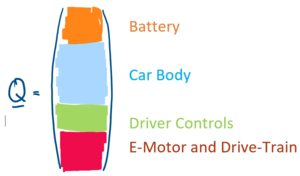
Each workpackage contributes state variables to the column vector q:
The IVP establishes mathematical equations describing how these state variables change over time, e.g. how a driver actuates the "gas"-pedal, which increases the motor-voltage, thus increasing the motor-torque and hence accelerating the car.
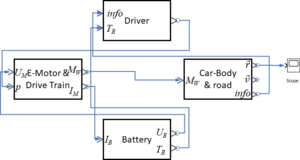
Our first approach is to depict each workpackage as graphical block and connect information / property exchange between blocks as in a diagramming tool:
The driver chooses a "gas"-pedal state "p" depending on information form the car's location, speed and battery temperature "TB". At the E-motor, "p" sets the nominal voltage "UM" of the E-motor, this implies a motor current "IM" and wheel torque "MW". The motor current "IM" then drives both the battery temperature and the available battery voltage "UB". And the wheel torque propels the car, delivering new locations and velocities. These are the submodels to be developed in each workpackage:
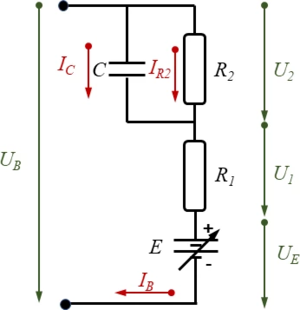
Battery
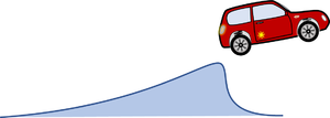
Car-Body
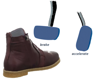
Driver-Controls
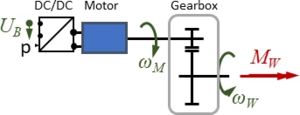
E-Motor and Drive-Train
Model
The mathematical model consists of XX differential equations with coordinates for each subsystem:
for the battery,
for the car-body
for the driver and
for the E-motor.
However, we have no elasticity accounted for between the E-motor and the wheel, thus
and so the remaining coordinates are
.
We have to deal with first and second order time derivatives of coordinates from q. All mechanical coordinates (e.g. ui, φ) are represented with their second-order time-derivatives that come from their D'Alembert's Inertia Forces. In order to transfer the equations of motion into a uniform set of differential equation of first order, we employ e.g.
so that the column matrix of state variables of the system is
.
But as indicated above the rotation angle of the front wheel ψM never appears in our equation - we remove it from the list of state variables.
Now in matrix-notation, the resultant equations of motion are
with
and
Simulation
Links
- ...
Literature
- ...
