Gelöste Aufgaben/JUMP: Unterschied zwischen den Versionen
Keine Bearbeitungszusammenfassung |
|||
| (37 dazwischenliegende Versionen desselben Benutzers werden nicht angezeigt) | |||
| Zeile 17: | Zeile 17: | ||
<onlyinclude> | <onlyinclude> | ||
[[Datei:JUMP-01.png|left|mini|Jump!]] | <table style="float: left"> | ||
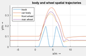
<tr><td>[[Datei:JUMP-01.png|left|mini|Jump!]]</td><td>[[Datei:JUMP-results-04c+.png|mini|170px|Trajectories]]</td></tr> | |||
</table> | |||
Create a mathematical Model for an RC-Model Car. | Create a mathematical Model for an RC-Model Car. | ||
| Zeile 68: | Zeile 70: | ||
And the wheel torque propels the car, delivering new locations and velocities. | And the wheel torque propels the car, delivering new locations and velocities. | ||
These are the submodels to be developed in each workpackage: | These are the submodels to be developed in each workpackage. Please follow the links: | ||
<div id="workpackages"> | <div id="workpackages"> | ||
| Zeile 216: | Zeile 218: | ||
in Matlab<sup>Ⓡ</sup> - the nonlinear characteristics and the algorithm that computes the contact points between car and track are too demanding for Maxima. | in Matlab<sup>Ⓡ</sup> - the nonlinear characteristics and the algorithm that computes the contact points between car and track are too demanding for Maxima. | ||
===Implementation in Matlab=== | ===Implementation in Matlab<sup>®</sup>=== | ||
We follow [[Werkzeuge/Software/Matlab/Grundstruktur eines | We follow [[Werkzeuge/Software/Matlab/Grundstruktur eines Matlab<sup>®</sup>-Programms|our basic process schema]] for implementing this initial-value-problem in Matlab<sup>®</sup>. | ||
The <nowiki>JUMP</nowiki>-script has these functions: | The <nowiki>JUMP</nowiki>-script has these functions: | ||
| Zeile 225: | Zeile 227: | ||
* post-processing. | * post-processing. | ||
Key to the solution process is a call to Matlab's own solver | Key to the solution process is a call to Matlab<sup>®</sup>'s own solver | ||
[https://la.mathworks.com/help/matlab/ref/ode15s.html ode15s] | [https://la.mathworks.com/help/matlab/ref/ode15s.html ode15s] | ||
| Zeile 237: | Zeile 239: | ||
The objects <nowiki>b, c, d, e, f</nowiki> are classes that hold parameters and functions related to each subsystem of the problem - from 'battery' to contact-'formulations'. | The objects <nowiki>b, c, d, e, f</nowiki> are classes that hold parameters and functions related to each subsystem of the problem - from 'battery' to contact-'formulations'. | ||
{{MyZipfileBlock|title=Matlab<sup>©</sup>-files| | {{MyZipfileBlock | ||
[[Datei: | |title=Matlab<sup>©</sup>-files | ||
|text =[[Datei:JUMP-folder-structure.png|links|mini|Folder Structure]]The folder-structure shows the main script <nowiki>JUMP.m</nowiki>. Classes and Functions are located in the respective dolfers. The Excel-file holds all system parameters. | |||
To download the full Matlab<sup>®</sup>-project download the zip-file from the link to your right. | |||
|file =JUMP.7z}} | |||
[[ | {{MySpreadsheetBlock | ||
|title=Systamparameter | |||
|text=[[Datei:JUMP-spreadsheet-tabs.png|links|mini|Tabs of the spreadsheet-file]]We collect all systems parameters in a spreadsheet file. Each system component has its own tab - e.g. the "car-body". We have two additional tabs, one for constants (gravity) and one for numerics (simulation end-time). | |||
|file=Params.xlsx}} | |||
Running the program will deliver these results: | |||
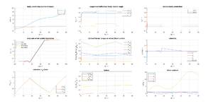
[[Datei:JUMP-results-01.png|mini|target speed: 10 m/s. (click to enlarge)|alternativtext=|ohne]]Take your time to study the individual diagrams. With such a high velocity prescribed, the integrator part of the controller is simply being filled up, the diagram to the lower right (row 3, column 3) shows that for "''E''". | |||
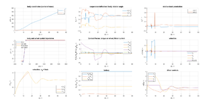
We'll investigate a few scenarios to the acquainted to the system, we start by reducing the target cruising speed to 2 m/s: | |||
[[Datei:JUMP-results-02.png|ohne|mini|target speed: 2 m/s]] | |||
Now our controller struggles to hold the prescribed speed downhill - remember, we have no breaks installed - and again on the steep climb upwards. But it works. | |||
Let's see what happens, if we beef-up the motor (higher M<sub>St</sub> and ω<sub>Nl</sub>) and switch-off the slip-control. We get a very different behaviour which shows our model-car speeding with screetching tires for 9 s < ''t'' < 15 s. | |||
[[Datei:JUMP-results-03.png|ohne|mini|target speed: 2 m/s]] | |||
As the highlight of this model, we want to let our model-car jump over a gap of - say ''L=3'' meters. | |||
We could try to simulate several combinations of initial values and system parameters to succeed - but that's too tiresome. We need to understand, what the "lift-off" velocity ''v<sub>0</sub>''on the ramp should be to make it to the other side. | |||
So let us define a ramp with an inclination of 1:10 thus a ramp angle of γ=atan(1/10), then a gap of three meters and then a ramp downwards - and ask for an analytical solution to the trajectory. | |||
Assuming - during the jump-phase - a motion of | |||
::<math>\begin{array}{ll} | |||
\underline{r}_C(t) &= \left(\begin{array}{c}u_1\\u_2\end{array}\right)\\ | |||
&= \left(\begin{array}{c}v_{0,x}+u_{1,0}\; t\\-\frac{1}{2} g \; t^2 + v_{0,y}\; t + u_{2,0}\end{array}\right) | |||
\end{array} | |||
</math>, | |||
which fulfills | |||
::<math>\begin{array}{ll} | |||
\underline{\ddot{r}}_C &= \left(\begin{array}{c}0\\-g\end{array}\right) | |||
\end{array} | |||
</math>, | |||
we find the boundary-conditions for the jump to be | |||
::<math>\begin{array}{ll} | |||
\underline{r}_C(0) &= \left(\begin{array}{c}0\\0\end{array}\right)\end{array} | |||
</math>, | |||
<math>\begin{array}{ll} | |||
\underline{\dot{r}}_C(0) &= \left(\begin{array}{c}v_0\; \cos(\gamma)\\v_0\; \sin(\gamma)\end{array}\right)\end{array} | |||
</math> | |||
and for the landing point | |||
<math>\begin{array}{ll} | |||
\underline{r}_C(t^*) &= \left(\begin{array}{c}L\\0\end{array}\right)\end{array} | |||
</math>. | |||
We compute that | |||
::<math>t^* = 0.2\;\frac{\displaystyle s^2}{\displaystyle m}\;v_0</math> and thus <math>v_0 = 12.3 \frac{\displaystyle m}{\displaystyle s}</math>, | |||
so we need to plan for a long run-up! | |||
===Simulation Runs=== | |||
We show a few examples of what can go wrong when doing this kind of simulations. | |||
I did not include the one where the car drives right through the ramp - because the stiff solver chose step-sizes which passed out on this object .... | |||
==== First "jump" attempt: a test-run ==== | |||
We select a speed-setpoint of ''V<sub>set</sub>'' = 1 m/s - and test the drive-range carefully. | |||
[[Datei:JUMP-results-04a.png|ohne|mini|Jump-attempt 1: easy test-run.]] | |||
Of course we did not jump - with such a low speed. We we know, the simulation performs as expected. | |||
==== Second "jump" attempt: ups - nearly made it ==== | |||
No we give full throttle: | |||
[[Datei:JUMP-results-04b.png|ohne|mini|Jump-attempt 2: crashed]] | |||
We did not just have the minimum speed to make the jump. Instead the car-model crashes into the ramp with its rear wheels and tips over. In our simulation it continues driving upside down - but with the car-body-center below the wheels. | |||
==== Third "jump" attempt: YES! ==== | |||
No we use a little more run-up and ... | |||
[[Datei:JUMP-results-04c.png|ohne|mini|Jump-attempt 3: YES!]] | |||
... yes - we made it! | |||
<hr/> | <hr/> | ||
Associated pages of the submodels: | |||
<splist showparent="no" | |||
sort="asc" | |||
sortby="title" | |||
liststyle="unordered" | |||
showpath="no" | |||
kidsonly="yes" | |||
debug="0" /> | |||
'''Links''' | '''Links''' | ||
Aktuelle Version vom 7. November 2021, 16:51 Uhr
Problem Statement
This example from Mechatronics combines mathematical models of mechanical and electrical components to simulate an RC-car-model. We've taken some reference-parameters from commercial vendors and adopted them as appropriate.
 |  |
Create a mathematical Model for an RC-Model Car.
The model shall account for the basic car-functions in a 2D-driving environment including vehicle dynamics, drive-train, battery and driver.
A 2D-test-parkour shall be provided to assess basic climbing and jumping capabilities of the car.
Overall Scope
We are tasked to provide a mathematical performance model for an RC-car model with a given reference-configuration. The mathematical model shall account for different operational envelopes and test for e.g. climbing capabilities, typical loads on springs and car-agility.
We follow a generic approach in modelling and simulation which consists of three overall steps:
- Structuring
- Modelling
- Simulating
Structure
The function of “structuring” is to break down this complex task - modelling and simulating the performance of our RC-car - into work-packages. We aim at reducing the complexity of the model until the remaining entities appears to be rather trivial to manage.
The structure we are aiming at is a pre-requisite for step 2: building the mathematical model. This model is the projection of the physical processes into mathematical equations. We’ll be implementing our model as an Initial-Value-Problem (IVP) , written in mathematical terms as
The left-hand side of the equation, q, are the state variables of our system. They are the minimum-set of values to describe the physical state of our model at a certain time t. The state variables stem from the car's sub-systems. We choose four workpackages to contribute to the state-variables:
- Battery:the power-source for the car
- Car Body: consisting of the car's chassis and its wheels
- Driver-Controls: processes that control acceleration and deceleration of the car
- E-Motor and Drive-Train: the mechanisms that transfer battery power into mechanical energy.
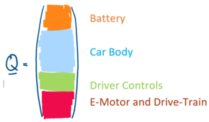
Each workpackage contributes state variables to the column vector q:
The IVP establishes mathematical equations describing how these state variables change over time, e.g. how a driver actuates the "gas"-pedal, which increases the motor-voltage, thus increasing the motor-torque and hence accelerating the car.
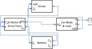
Our first approach is to depict each workpackage as graphical block and connect information / property exchange between blocks as in a diagramming tool:
The driver chooses a "gas"-pedal state "p" depending on information form the car's location, speed and battery temperature "TB".
At the E-motor, "p" sets the nominal voltage "UM" of the E-motor, this implies a motor current "IM" and wheel torque "MW".
The motor current "IM" then drives both the battery temperature and the available battery voltage "UB".
And the wheel torque propels the car, delivering new locations and velocities.
These are the submodels to be developed in each workpackage. Please follow the links:
Model
The mathematical model consists of XX differential equations with coordinates for each subsystem:
- for the battery,
- for the car-body
- for the driver and
- for the E-motor.
However, we have no elasticity accounted for between the E-motor and the wheel, thus
and so the remaining coordinates are
- .
We have to deal with first and second order time derivatives of coordinates from q. All mechanical coordinates (e.g. ui, φ) are represented with their second-order time-derivatives that come from their D'Alembert's Inertia Forces. In order to transfer the equations of motion into a uniform set of differential equation of first order, we employ e.g.
so that the column matrix of state variables of the system is
- .
But as indicated above the rotation angle of the front wheel ψM never appears in our equation - we remove it from the list of state variables.
Now in matrix-notation, the resultant equations of motion are
with
and
Simulation
We implement the system of differential equations
in MatlabⓇ - the nonlinear characteristics and the algorithm that computes the contact points between car and track are too demanding for Maxima.
Implementation in Matlab®
We follow [[Werkzeuge/Software/Matlab/Grundstruktur eines Matlab®-Programms|our basic process schema]] for implementing this initial-value-problem in Matlab®.
The JUMP-script has these functions:
- pre-processing,
- solving and
- post-processing.
Key to the solution process is a call to Matlab®'s own solver
ode15s
for stiff differential equations. Though the equations of motion are not intrinsically stiff, this solver provided the best performance if the car encounters e.g. a rough touch-down after a jump-phase. The call to ode15s is
[t,y] = ode15s(@(t,y)jumpdydt(t,y,parC,parN,b,c,d,e,f),tspan,y0);
with parC, parN being maps of parameters.
The objects b, c, d, e, f are classes that hold parameters and functions related to each subsystem of the problem - from 'battery' to contact-'formulations'.
Matlab©-files

The folder-structure shows the main script JUMP.m. Classes and Functions are located in the respective dolfers. The Excel-file holds all system parameters.
To download the full Matlab®-project download the zip-file from the link to your right.

download compressed archive →
Systamparameter

We collect all systems parameters in a spreadsheet file. Each system component has its own tab - e.g. the "car-body". We have two additional tabs, one for constants (gravity) and one for numerics (simulation end-time).

download spreadsheet →
Running the program will deliver these results:
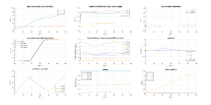
Take your time to study the individual diagrams. With such a high velocity prescribed, the integrator part of the controller is simply being filled up, the diagram to the lower right (row 3, column 3) shows that for "E".
We'll investigate a few scenarios to the acquainted to the system, we start by reducing the target cruising speed to 2 m/s:
Now our controller struggles to hold the prescribed speed downhill - remember, we have no breaks installed - and again on the steep climb upwards. But it works.
Let's see what happens, if we beef-up the motor (higher MSt and ωNl) and switch-off the slip-control. We get a very different behaviour which shows our model-car speeding with screetching tires for 9 s < t < 15 s.
As the highlight of this model, we want to let our model-car jump over a gap of - say L=3 meters. We could try to simulate several combinations of initial values and system parameters to succeed - but that's too tiresome. We need to understand, what the "lift-off" velocity v0on the ramp should be to make it to the other side.
So let us define a ramp with an inclination of 1:10 thus a ramp angle of γ=atan(1/10), then a gap of three meters and then a ramp downwards - and ask for an analytical solution to the trajectory.
Assuming - during the jump-phase - a motion of
- ,
which fulfills
- ,
we find the boundary-conditions for the jump to be
- ,
and for the landing point .
We compute that
- and thus ,
so we need to plan for a long run-up!
Simulation Runs
We show a few examples of what can go wrong when doing this kind of simulations. I did not include the one where the car drives right through the ramp - because the stiff solver chose step-sizes which passed out on this object ....
First "jump" attempt: a test-run
We select a speed-setpoint of Vset = 1 m/s - and test the drive-range carefully.
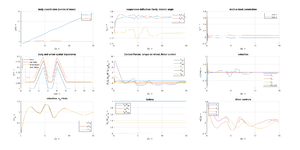
Of course we did not jump - with such a low speed. We we know, the simulation performs as expected.
Second "jump" attempt: ups - nearly made it
No we give full throttle:
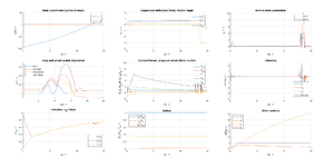
We did not just have the minimum speed to make the jump. Instead the car-model crashes into the ramp with its rear wheels and tips over. In our simulation it continues driving upside down - but with the car-body-center below the wheels.
Third "jump" attempt: YES!
No we use a little more run-up and ...
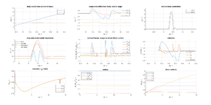
... yes - we made it!
Associated pages of the submodels:
Links
- ...
Literature
- ...