Gelöste Aufgaben/JUMP/Driver Controls: Unterschied zwischen den Versionen
K →Model |
|||
| (9 dazwischenliegende Versionen desselben Benutzers werden nicht angezeigt) | |||
| Zeile 27: | Zeile 27: | ||
==Model== | ==Model== | ||
The most common controller in technical applications is a [[wikipedia:PID_controller|PID-controller]]. Our target value to control is ''v<sub>rel</sub>'' | The most common controller in technical applications is a [[wikipedia:PID_controller|PID-controller]] which are based on the proportional, integral, and derivative terms of the error-value. Our target value to control is both | ||
<ul> | |||
<li>the slip-velocity ''v<sub>rel</sub>'' with set-point <math>r := v_\epsilon</math> and</li> | |||
<li>the cruising-velocoty ''v<sub>c</sub>'' with set-point <math>r := V_{set}</math>.</li> | |||
</ul> | |||
We define the error values <u>e</u> for both as | |||
and | ::<math>\begin{array}{ll} | ||
e_1 &= f_1(\tilde{v}) \text{ with } \tilde{v} = \frac{\displaystyle v_{rel}}{\displaystyle v_{\varepsilon}}; \text{ here we choose }\\ | |||
&= 1+\tilde{v} | |||
\end{array}</math> | |||
and | |||
::<math>\begin{array}{ll} | ::<math>\begin{array}{ll} | ||
e_2 &= f_2(\tilde{v}) \text{ with } \tilde{v} = \frac{\displaystyle v_{c}}{\displaystyle V_{set}}; \text{ here we choose }\\ | |||
&= 1-\tilde{v} | &= 1-\tilde{v} | ||
\end{array}</math> . | \end{array}</math>. | ||
The functions for ''e<sub>1</sub>'' ensures that "''p"'' increases e.g. if ''v<sub>rel</sub>'' < ''v<sub>ε</sub>'' and decreases otherwise. [[Datei:JUMP-driver-blockdiagram-controller.png|mini|Block-diagram controller]]With controller parameters ''K<sub>p</sub>, Ki, K<sub>d</sub>'' we get this diagram for the controlled system. | |||
When increasing the speed to target-value ''V<sub>set</sub>'', the maximum force delivered at the point of contact ''C'' governs the acceleration of the car-body. | |||
Thus, we set the relevant error-value to be | |||
::<math>\tilde{e} := \min(e_1, e_2)</math> | |||
The | The controller thus adds to the state variable | ||
::<math>E_I := \displaystyle \int_0^t \tilde{e}(\tau) d\tau</math> | |||
of the system. | |||
For the differentiator-part we would need to find | |||
::<math>\begin{array}{ll} | ::<math>\begin{array}{ll} | ||
\dot{e} &= \frac{\displaystyle \ | \dot{e} &= \frac{\displaystyle d\, e(t)}{\displaystyle d\, t}\\ | ||
&=\frac{\displaystyle 1}{\displaystyle v_{red}} \cdot \frac{\displaystyle d v_{rel}(t)}{\displaystyle d t}\\ | &=\frac{\displaystyle 1}{\displaystyle v_{red}} \cdot \frac{\displaystyle d v_{rel}(t)}{\displaystyle d t}\\ | ||
\end{array}</math> | \end{array}</math> | ||
| Zeile 57: | Zeile 73: | ||
::<math>\underline{q}_D(t) = \left(E(t)\right)</math> . | ::<math>\underline{q}_D(t) = \left(E(t)\right)</math> . | ||
The output "p" of the submodel is not a state variable, but | The output "p" of the submodel is not directly a state variable, but | ||
::<math>p^*(t) = K_p\cdot e(t) + K_i\cdot E(t) + K_d\cdot \dot{e}(t) </math> | |||
But since the DC/DC-converter can only take values between 0 ... 1 we define | |||
::<math>p(t) = \min(\max(p^*,0),1)</math> | |||
This constraint in the value of ''p'' brings more headache to the problem, because the integrator-part ''E''of the controller "runs-off" if the error-value <math>\tilde{e} := min(e_1, e_2)</math> is positive for a long period of the simulation. We'll see that later. | |||
==Variables== | ==Variables== | ||
| Zeile 76: | Zeile 98: | ||
!name | !name | ||
!symbol | !symbol | ||
!value | |||
!unit | !unit | ||
|- | |- | ||
|coefficient of proportional contribution | |coefficient of proportional contribution | ||
|''K<sub>p</sub>'' | |''K<sub>p</sub>'' | ||
|1 | |||
|1/s | |1/s | ||
|- | |- | ||
|coefficient of integrator contribution | |coefficient of integrator contribution | ||
|''K<sub>i</sub>'' | |''K<sub>i</sub>'' | ||
|100 | |||
|1/s^2 | |1/s^2 | ||
|- | |- | ||
|coefficient of differential contribution | |coefficient of differential contribution - not employed | ||
|''K<sub>d</sub>'' | |''K<sub>d</sub>'' | ||
| | |||
|1 | |1 | ||
|- | |||
|max. tolerated battery temperature | |||
|''T<sub>B,max</sub>'' | |||
|60 | |||
|°C | |||
|- | |||
|target-speed (choose very high when you want "pedal to the metal") | |||
|''V<sub>set</sub>'' | |||
|10 | |||
|m/s | |||
|} | |} | ||
Aktuelle Version vom 22. März 2021, 15:46 Uhr

Since we’re in a 2D-simulation environment, the driver controls only “gas” (acceleration) and breaks - no directional control needed to be taken into account.
Scope

The track poses challenges that require the driver to control the driving and breaking torque on the wheel. These track-specific challenges include
- achieving maximum acceleration, thus avoiding wheel-skid and adjusting to a slip that provides optimal traction,
- achieving maximum deceleration when breaking and therefore avoiding wheels becoming locked,
- avoiding excessive battery-temperatures and thus controlling driving torque.
Structure
The driver is tasked to control wheel slip and wheel skid via the "gas"-pedal. We differentiate between
- slip as the relative micro-velocity necessary to transmit forces in rolling contact and
- skip as unwanted excessive relative velocity resulting from poor torque-control at the wheels.
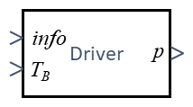
The information for this task come as "info" from the car's motion.

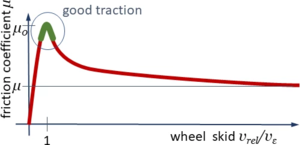
To avoid wheel skid and to control slip, the driver will aim to maintain a relative velocity at the wheel-contact point “C“ around the small velocity vε, thus reducing torque MW if vrel > vε and increasing MW if vrel < vε.
This is a very challenging system to be controlled because
- the velocity domain that we target is rather small and
- the characteristic for vrel > vε is degressive: the friction force decreases with relative velocity.
Model
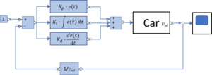
The most common controller in technical applications is a PID-controller which are based on the proportional, integral, and derivative terms of the error-value. Our target value to control is both
- the slip-velocity vrel with set-point and
- the cruising-velocoty vc with set-point .
We define the error values e for both as
and
- .
The functions for e1 ensures that "p" increases e.g. if vrel < vε and decreases otherwise.

With controller parameters Kp, Ki, Kd we get this diagram for the controlled system.
When increasing the speed to target-value Vset, the maximum force delivered at the point of contact C governs the acceleration of the car-body. Thus, we set the relevant error-value to be
The controller thus adds to the state variable
of the system.
For the differentiator-part we would need to find
as the rate of change from the Car-Body-Model.
So the only state variable from the driver is
- .
The output "p" of the submodel is not directly a state variable, but
But since the DC/DC-converter can only take values between 0 ... 1 we define
This constraint in the value of p brings more headache to the problem, because the integrator-part Eof the controller "runs-off" if the error-value is positive for a long period of the simulation. We'll see that later.
Variables
| name | symbol | unit |
|---|---|---|
| integrator part of PID controller | E(t) | 1 |
Parameter
| name | symbol | value | unit |
|---|---|---|---|
| coefficient of proportional contribution | Kp | 1 | 1/s |
| coefficient of integrator contribution | Ki | 100 | 1/s^2 |
| coefficient of differential contribution - not employed | Kd | 1 | |
| max. tolerated battery temperature | TB,max | 60 | °C |
| target-speed (choose very high when you want "pedal to the metal") | Vset | 10 | m/s |
next workpackage: e-motor and drive-train →
References
- Yuan, Lei; Chen, Hong; Ren, Bingtao; Zhao, Haiyan: Model predictive slip control for electric vehicle with four in-wheel motors, Proceedings of the 34th Chinese Control Conference July 28-30, 2015, Hangzhou, China, p 7895-7900
- ...