Gelöste Aufgaben/UEBI: Unterschied zwischen den Versionen
Die Seite wurde neu angelegt: „h“ |
Keine Bearbeitungszusammenfassung |
||
| (23 dazwischenliegende Versionen desselben Benutzers werden nicht angezeigt) | |||
| Zeile 1: | Zeile 1: | ||
h | [[Category:Gelöste Aufgaben]] | ||
[[Category:Dimensionslose Schreibweise]] | |||
[[Category:Analytische Lösung]] | |||
[[Category:Randwertproblem]] | |||
[[Category:Biege-Belastung]][[Category:Euler-Bernoulli-Balken]] | |||
[[Category:Maxima]] | |||
==Aufgabenstellung== | |||
Der Euler-Bernoulli-Balken ''AB'' wird durch seine Gewichtskraft belastet. Er ist in ''A'' fest eingespannt und hat eine konstante Breite b sowie eine zwischen A und B linear veränderliche Höhe ''h''. | |||
In [[Gelöste Aufgaben/UEBF|UEBF]] haben wir eine Näherungslösung für dieses Problem berechnet. | |||
<onlyinclude> | |||
[[Datei:UEBF-01.png|alternativtext=|links|mini|200x200px|Lageplan]] | |||
Gesucht ist die analytische Lösung des Problems. | |||
</onlyinclude> | |||
Gegeben sind für den Balken: | |||
* Länge ''ℓ'', Breite ''b,'' | |||
* E-Modul ''E'', Dichte ''ρ'' und | |||
* die Höhe ''h''<sub>0</sub>''=b'' und ''h<sub>1</sub>'' jeweils in ''A'' und ''B''; dazwischen ist die Höhe linear veränderlich. | |||
== Lösung mit Maxima == | |||
Um zur analytischen Lösung zukommen, müssen wir berücksichtigen, dass | |||
::<math>E\,I(x) \cdot \displaystyle \frac{d^2}{dx^2}w(x) = -M(x)</math>. | |||
Wir müssen also hier die Abhängigkeit der Querschnittseigenschaften von "''x''" in der Differentialbeziehung berücksichtigen. Das macht die Sache deutlich komplizierter als vorher. | |||
<!--------------------------------------------------------------------------------> | |||
{{MyCodeBlock|title=Header | |||
|text= | |||
Wir haben die Differential-Beziehungen | |||
::<math>\begin{array}{rcl} | |||
Q' &=&-q\\ | |||
M' &=&+Q\\ | |||
E\,I\cdot\phi' &=& -M\\ | |||
w' &=&+\phi | |||
\end{array}</math> | |||
für die Querkraft ''Q'', das Moment ''M'', die Verkippung der Querschnitte ''ϕ'' und die Auslenkung ''w''. Dabei ist die ortsabhängige Streckenlast | |||
::<math>q(x) = A(x)\, \rho \, g \text{ mit } A(x) = b \cdot h(x).</math> | |||
Die Höhe des Balkens ist linear veränderlich, nämlich | |||
::<math>h(x) = h_0\, (1-\xi) + h_1 \, \xi \text{ mit } \xi = \displaystyle \frac{x}{\ell}</math>. | |||
|code= | |||
<syntaxhighlight lang="lisp" line start=1> | |||
/*******************************************************/ | |||
/* MAXIMA script */ | |||
/* version: wxMaxima 18.10.1 */ | |||
/* author: Andreas Baumgart */ | |||
/* last updated: 2019-09-30 */ | |||
/* ref: TM-C, Balken mit linear-veränderlicher Höhe */ | |||
/* description: finds the analytic solution for */ | |||
/* problem */ | |||
/*******************************************************/ | |||
/* declare variational variables - see 6.3 Identifiers */ | |||
declare( "ℓ", alphabetic); | |||
declare( "ϕ", alphabetic); | |||
</syntaxhighlight> | |||
}} | |||
<!--------------------------------------------------------------------------------> | |||
{{MyCodeBlock|title=Declarations | |||
|text= | |||
Diese Abkürzungen führen wir ein: | |||
::<math>\displaystyle m = \rho\,\frac{h_0+h_1}{2}\,b \, \ell \, g</math>, | |||
::<math>h_1 = \alpha \, h_0</math>. | |||
Für die Ergebnisse setzten wir dann exemplarisch | |||
::<math>\displaystyle \alpha = \frac{1}{2}</math> | |||
an - sonst werden die Ausdrücke zu umfangreich. | |||
|code= | |||
<syntaxhighlight lang="lisp" line start=1> | |||
/* make equations of motion dim'less with load case #6 */ | |||
reference : [Phi[ref] = W[ref]/ℓ, W[ref] = q[ref]*ℓ^4/(8*E I[ref]), | |||
M[ref] = m*g*ℓ, Q[ref] = m*g, | |||
q[ref] = m*g/ℓ, EI[ref]=E*b*((H[0]+H[1])/2)^3/12]; | |||
/* system parameters */ | |||
params: [q[0] = A(xi)*rho*g, | |||
A(xi) = b*h(xi), | |||
I(xi) = b*h(xi)^3/12, | |||
h(xi) = H[0]*(1-xi)+ H[1]*xi]; | |||
params: append(params, | |||
solve((H[0]+H[1])/2*b*ℓ*rho=m, rho)); | |||
geometry : [alpha=1/2]; | |||
dimless: [x = xi*ℓ, H[0]=b, H[1]=alpha*b]; | |||
sections: [%c4=C[0], %c3=C[1], %c2=C[2], %c1=C[3]]; | |||
</syntaxhighlight> | |||
}} | |||
<!--------------------------------------------------------------------------------> | |||
{{MyCodeBlock|title=Dimensionless Form of Differential Equations | |||
|text= | |||
Beim Aufintegrieren der Differentialgleichungen stören die vielen dimensionsbehafteten Parameter. Viel einfacher werden die Gleichungen, wenn wir sie in dimensionsloser Form - mit dimensionsloser Auslenkung, Kippwinkel, Biegemoment und Querkraft anschreiben, also | |||
::<math>\begin{array}{lcc} | |||
w &= W_{ref}&\cdot& \tilde{w}\\ | |||
\phi &= \Phi_{ref}&\cdot& \tilde{\phi}\\ | |||
M &= M_{ref}&\cdot& \tilde{M}\\ | |||
Q &= Q_{ref}&\cdot& \tilde{Q} | |||
\end{array}</math>. | |||
Wir wählen dazu als Referenzlösung den [[Sources/Lexikon/Euler-Bernoulli-Balken/Standard-Lösungen#Kragbalken Streckenlast|Kragbalken mit konstantem Querschnitt unter konstanter Streckenlast]], mit der maximalen Auslenkung | |||
::<math>W_{ref} = \displaystyle \frac{q_{ref} \, \ell^4}{8\,E\,I_{ref}}</math>. | |||
Als Referenz-Werte für die Streckenlast wählen wir hier die Werte unseres Balkens in ''x=ℓ/2'', demnach | |||
::<math>\begin{array}{ll} | |||
q_{ref} &= A_{ref}\,\rho\,g \text{ mit } A_{ref} = b\cdot h(\displaystyle\frac{\ell}{2})\\ | |||
I_{ref} & = \displaystyle \frac{b\cdot h(\displaystyle\frac{\ell}{2})^3}{12} | |||
\end{array}</math>. | |||
Die Differentialgleichungen werden dadurch und mit der dimensionslosen Ortskoordinate | |||
::<math>\xi = \displaystyle\frac{x}{\ell}</math> | |||
viel einfacher, nämlich | |||
::<math>\begin{array}{rcl} | |||
\displaystyle \frac{\partial}{\partial\xi}\tilde{Q} &=& - \displaystyle\frac{4-2\xi}{3}\\ | |||
\frac{\displaystyle\partial}{\displaystyle\partial\xi} \tilde{M} &=&+\tilde{Q}\\ | |||
\frac{\displaystyle\partial}{\displaystyle\partial\xi} \tilde{\phi} &=&-\frac{\displaystyle 8}{\frac{I(\displaystyle \xi)}{\displaystyle I_{ref}}}\cdot \tilde{M} \text{ mit } \frac{\displaystyle I(\xi)}{\displaystyle I_{ref}} = \frac{\displaystyle (\alpha+1)^3}{\displaystyle 8\,((\alpha-1)\,\xi+1)^3}\\ | |||
\frac{\displaystyle \partial}{\displaystyle \partial\xi} \tilde{w} &=&+\tilde{\phi} | |||
\end{array}</math>. | |||
Damit es übersichtlicher wird, lassen wir die Tilden über den gesuchten dimensionslosen Funktionen gleich wieder weg. | |||
|code= | |||
<syntaxhighlight lang="lisp" line start=1> | |||
/******************************************************/ | |||
/* Boundary Value Problem Formulation */ | |||
/* field */ | |||
dgl : [ Q[ref]*diff(Q(xi),xi)/ℓ = - q(xi), | |||
M[ref]*diff(M(xi),xi)/ℓ = + Q[ref]*Q(xi), | |||
E*I(xi)*diff(Phi[ref]*ϕ(xi),xi)/ℓ = - M[ref]*M(xi), | |||
diff(W[ref]*w(xi),xi)/ℓ = + Phi[ref]*ϕ(xi)]; | |||
dgl: subst(reference,dgl); | |||
</syntaxhighlight> | |||
}} | |||
<!--------------------------------------------------------------------------------> | |||
{{MyCodeBlock|title=Integration Of Differential Equation | |||
|text= | |||
Die Differentialbeziehungen lösen wir nun sukzessive zu | |||
::<math>\displaystyle Q(\xi)=\frac{\xi^2 - 4 \xi + 3\,C_3}{3}</math>, | |||
::<math>\displaystyle M(\xi)= \frac{{{\xi}^{3}}-6 {{\xi}^{2}}+9 {C_3} \xi+9 {C_2}}{9}</math>. | |||
Bis hier ist alles wie gehabt - aber jetzt steht das ortsveränderliche Flächenmoment ''I(ξ)'' im Nenner. Maxima liefert | |||
::<math>\displaystyle \phi(\xi)) = \frac{6 {{\xi}^{3}}+\left( 2 {C_1}-24\right) \, {{\xi}^{2}}+\left( -54 {C_3}-8 {C_1}+96\right) \xi+54 {C_3}-27 {C_2}+8 {C_1}-96}{2 {{\xi}^{2}}-8 \xi+8}</math> | |||
und im nächsten Schritt schließlich | |||
::<math>\displaystyle w(\xi) = \frac{3 {{\xi}^{3}}+\left( 2 {C_1}-6\right) \, {{\xi}^{2}}+\left( \left( 72-54 {C_3}\right) \ln{\displaystyle \left( -\frac{\xi-2}{2}\right) }-4 {C_1}+2 {C_0}\right) \xi+\left( 108 {C_3}-144\right) \ln{\displaystyle \left( -\frac{\xi-2}{2}\right) }+54 {C_3}+27 {C_2}-4 {C_0}-48}{2 \xi-4}</math>. | |||
Darin enthalten sind die unbekannten - also gesuchten - Integrationskonstanten | |||
::<math>C_0, C_1, C_2, C_3</math>. | |||
|code= | |||
<syntaxhighlight lang="lisp" line start=1> | |||
/******************************************************/ | |||
/* integrate differential equations */ | |||
displ : ratsimp(integrate(subst(dimless,ratsimp(subst(params,solve(dgl[1],Q(xi))))),xi)); | |||
displ : append(displ, ratsimp(integrate(subst(displ,solve(dgl[2],M(xi))),xi))); | |||
displ : append(displ, ratsimp( | |||
integrate( | |||
ratsimp(subst(dimless,subst(geometry,subst(displ, subst(params,solve(dgl[3],'diff(ϕ(xi),xi))))))),xi | |||
))); | |||
displ : append(displ, ratsimp( | |||
integrate( | |||
subst(displ, | |||
solve(dgl[4],w(xi)) | |||
), | |||
xi))); | |||
displ : ratsimp(subst(sections, subst(geometry,displ))); | |||
</syntaxhighlight> | |||
}} | |||
<!--------------------------------------------------------------------------------> | |||
{{MyCodeBlock|title=Boundary Conditions | |||
|text=Diese Unbekannten bestimmen wir aus den Randbedingungen, nämlich | |||
::<math>\begin{array}{rcl} | |||
w(0) &=& 0\\ | |||
\phi(0) &=& 0\\ | |||
M(1) &=& 0\\ | |||
Q(1) &=& 0\\ | |||
\end{array}</math> | |||
und damit | |||
::<math>\begin{array}{rcl} | |||
0&=&C_3-1\\ | |||
0&=&9 {C_3}+9 {C_2}-5\\ | |||
0&=&54 {C_3}-27 {C_2}+8 {C_1}-96\\ | |||
0&=&-54 {C_3}-27 {C_2}+4 {C_0}+48 | |||
\end{array} | |||
</math>. | |||
|code= | |||
<syntaxhighlight lang="lisp" line start=1> | |||
/******************************************************/ | |||
/* part II: boundary conditions */ | |||
node[A]: [ w(0) = 0, | |||
ϕ(0) = 0]; | |||
node[B]: [ Q(1) = 0, | |||
M(1) = 0]; | |||
BCs : [subst(node[B],subst([xi=1],displ[1])), | |||
subst(node[B],subst([xi=1],displ[2])), | |||
subst(node[A],subst([xi=0],displ[3])), | |||
subst(node[A],subst([xi=0],displ[4]))]; | |||
scale: [3, 9, 8, 4]; | |||
BCs : expand(ratsimp(scale*BCs)); | |||
</syntaxhighlight> | |||
}} | |||
<!--------------------------------------------------------------------------------> | |||
{{MyCodeBlock|title=Solving | |||
|text= | |||
Zum Lösen bringen wir die Gleichungen in die Form | |||
::<math>\begin{pmatrix}0 & 0 & 0 & -3\\ | |||
0 & 0 & -9 & -9\\ | |||
0 & -8 & 27 & -54\\ | |||
-4 & 0 & 27 & 54\end{pmatrix} | |||
\cdot \begin{pmatrix}{C_0}\\ | |||
{C_1}\\ | |||
{C_2}\\ | |||
{C_3}\end{pmatrix} = \begin{pmatrix}-3\\ | |||
-5\\ | |||
-96\\ | |||
48\end{pmatrix}</math>, | |||
die wir lösen zu | |||
::<math>\begin{array}{lcc} | |||
C_0&=& - \displaystyle\frac{3}{2},\\ | |||
C_1&=& + \displaystyle\frac{15}{4},\\ | |||
C_2&=& - \displaystyle\frac{4}{9},\\ | |||
C_3&=& + 1 | |||
\end{array}</math>. | |||
|code= | |||
<syntaxhighlight lang="lisp" line start=1> | |||
/* integration constants = unknowns */ | |||
X : [C[0],C[1],C[2],C[3]]; | |||
ACM: augcoefmatrix(BCs,X); | |||
/* system matrix and rhs */ | |||
AA : submatrix(ACM,5); | |||
bb : - col(ACM,5); | |||
/* print OLE */ | |||
print(subst(params,AA),"*",transpose(X),"=",subst(params,bb))$ | |||
/******************************************************/ | |||
/* solving */ | |||
D : ratsimp(determinant(AA))$ | |||
[ P, L, U] : ratsimp(get_lu_factors(lu_factor(AA)))$ | |||
cc : ratsimp(linsolve_by_lu(AA,bb)[1])$ | |||
sol : makelist(X[i] = cc[i][1],i,1,4)$ | |||
</syntaxhighlight> | |||
}} | |||
<!--------------------------------------------------------------------------------> | |||
{{MyCodeBlock|title=Post-Processing | |||
|text= | |||
Die Ergebnisse schauen wir uns in dimensionsloser Form an, wobei wir die Standard-Lösungen für den Balken unter konstanter Streckenlast ansetzen. | |||
Für | |||
::<math>\begin{array}{lcl} | |||
W_{ref} &=& \displaystyle \frac{q_{ref}\cdot \ell^4}{8 EI_{ref}},\\ | |||
\Phi_{ref} &=& \displaystyle \frac{W_{ref}}{\ell},\\ | |||
M_{ref} &=& m\cdot g\cdot \ell,\\ | |||
Q_{ref} &=& m\cdot g,\\ | |||
q_{ref} &=& m\cdot g/\ell,\\ | |||
EI_{ref} &=& E\cdot \displaystyle \frac{b\cdot ((H_{0}+H_{1})/2)^3}{12} | |||
\end{array}</math> | |||
finden wir | |||
<ul> | |||
<li>... für ''w(ξ)'': | |||
[[Datei:UEBI-31.png|mini|Auslenkung ''w(x)''|alternativtext=|ohne]]</li> | |||
<li>... für ''ϕ(ξ)'': | |||
[[Datei:UEBI-32.png|mini|Querschnitts-Kippung ''w'(x)''|alternativtext=|ohne]]</li> | |||
<li>... für ''M(ξ)'': | |||
[[Datei:UEBI-33.png|mini|Momentenverlauf ''M(x)''|alternativtext=|ohne]]</li> | |||
<li>... für ''Q(ξ)'': | |||
[[Datei:UEBI-34.png|mini|Querkraftverlauf ''Q(x)''|alternativtext=|ohne]]</li> | |||
</ul> | |||
|code= | |||
<syntaxhighlight lang="lisp" line start=1> | |||
/******************************************************/ | |||
/* post-processing */ | |||
/* bearing forces and moments */ | |||
reactForces: [M[A] = M[ref]*M(0), | |||
Q[z] = Q[ref]*Q(0)]; | |||
reactForces: ratsimp(subst(sol, subst(subst([xi=0],displ),subst(reference,reactForces)))); | |||
/* plot displacements */ | |||
fcts: [ w (xi), | |||
ϕ (xi), | |||
M (xi), | |||
Q (xi)]; | |||
textlabels : ["← w(x)/w[rez]", "← w'(x)/ϕ[ref]", "M(x)/(m*g*ℓ) →", "Q(x)/(m g) →"]; | |||
for i: 1 thru 4 do( | |||
f : ratsimp(subst(geometry,subst(sol, subst(geometry,subst(dimless,subst(displ,subst(params,fcts[i]))))))), | |||
preamble: if i<=2 then "set yrange [] reverse" else "set yrange []", | |||
plot2d(f, [xi,0,1], [legend, false], | |||
[gnuplot_preamble, preamble], | |||
[xlabel, "x/ℓ →"], | |||
[ylabel, textlabels[i]]) )$ | |||
/******************************************************/ | |||
/* print tabular values */ | |||
for i: 1 thru 4 do( | |||
f : ratsimp(subst(geometry,subst(sol, subst(geometry,subst(dimless,subst(displ,subst(params,fcts[i])))))*facts[i])), | |||
N :100, | |||
print("table for",textlabels[i]), | |||
for j: 0 thru N do ( | |||
t : j/N, | |||
print(float(t),";",expand(float(subst([xi=t],f)))) | |||
))$ | |||
</syntaxhighlight> | |||
}} | |||
===Plot Data=== | |||
{{MyDataBlock | |||
|title=Datenpunkte der Auslenkung ''w(ξ)'' | |||
|text=Die Tabelle enthält die Werte ''ξ'' und ''w(ξ)'' zum Herunterladen. | |||
|data= | |||
<syntaxhighlight lang="Clean" line start=1 style="border:3px dashed gray"> | |||
table for ← w(x)/w[rez] | |||
0.0 ; 0.0 | |||
0.01 ; 7.481203031248985*10^-5 | |||
0.02 ; 2.984924700020887*10^-4 | |||
0.03 ; 6.698993034749879*10^-4 | |||
0.04 ; 0.001187879040283986 | |||
0.05 ; 0.00185126660292937 | |||
0.06 ; 0.002658885214942354 | |||
0.07 ; 0.003609546289359847 | |||
0.08 ; 0.004702049317703514 | |||
0.09 ; 0.005935181759589655 | |||
0.1 ; 0.007307718933097404 | |||
0.11 ; 0.008818423906038287 | |||
0.12 ; 0.01046604738827592 | |||
0.13 ; 0.01224932762526032 | |||
0.14 ; 0.01416699029293324 | |||
0.15 ; 0.01621774839421548 | |||
0.16 ; 0.01840030215723649 | |||
0.17 ; 0.02071333893554073 | |||
0.18 ; 0.02315553311047674 | |||
0.19 ; 0.02572554599601331 | |||
0.2 ; 0.02842202574623001 | |||
0.21 ; 0.03124360726574977 | |||
0.22 ; 0.03418891212340282 | |||
0.23 ; 0.0372565484694203 | |||
0.24 ; 0.04044511095649053 | |||
0.25 ; 0.04375318066501066 | |||
0.26 ; 0.04717932503291399 | |||
0.27 ; 0.05072209779045508 | |||
0.28 ; 0.0543800389003753 | |||
0.29 ; 0.05815167450388911 | |||
0.3 ; 0.06203551687296655 | |||
0.31 ; 0.06603006436941357 | |||
0.32 ; 0.07013380141128575 | |||
0.33 ; 0.07434519844720817 | |||
0.34 ; 0.07866271193920962 | |||
0.35 ; 0.08308478435471277 | |||
0.36 ; 0.08760984416838222 | |||
0.37 ; 0.09223630587454254 | |||
0.38 ; 0.09696257001097904 | |||
0.39 ; 0.1017870231949183 | |||
0.4 ; 0.1067080381721125 | |||
0.41 ; 0.1117239738799426 | |||
0.42 ; 0.1168331755255615 | |||
0.43 ; 0.1220339746801493 | |||
0.44 ; 0.1273246893904267 | |||
0.45 ; 0.1327036243086318 | |||
0.46 ; 0.1381690708422802 | |||
0.47 ; 0.1437193073250795 | |||
0.48 ; 0.1493525992104727 | |||
0.49 ; 0.1550671992894059 | |||
0.5 ; 0.160861347933972 | |||
0.51 ; 0.1667332733687484 | |||
0.52 ; 0.1726811919717323 | |||
0.53 ; 0.1787033086069086 | |||
0.54 ; 0.1847978169906433 | |||
0.55 ; 0.1909629000942185 | |||
0.56 ; 0.1971967305850093 | |||
0.57 ; 0.2034974713089322 | |||
0.58 ; 0.2098632758170441 | |||
0.59 ; 0.2162922889392689 | |||
0.6 ; 0.2227826474085497 | |||
0.61 ; 0.229332480538859 | |||
0.62 ; 0.2359399109607717 | |||
0.63 ; 0.2426030554186048 | |||
0.64 ; 0.2493200256333157 | |||
0.65 ; 0.2560889292357581 | |||
0.66 ; 0.2629078707751271 | |||
0.67 ; 0.2697749528078152 | |||
0.68 ; 0.2766882770722823 | |||
0.69 ; 0.2836459457558966 | |||
0.7 ; 0.2906460628602184 | |||
0.71 ; 0.2976867356715562 | |||
0.72 ; 0.3047660763442248 | |||
0.73 ; 0.3118822036044391 | |||
0.74 ; 0.3190332445833526 | |||
0.75 ; 0.3262173367883804 | |||
0.76 ; 0.3334326302226785 | |||
0.77 ; 0.340677289663329 | |||
0.78 ; 0.3479494971096025 | |||
0.79 ; 0.3552474544135462 | |||
0.8 ; 0.3625693861060849 | |||
0.81 ; 0.3699135424327804 | |||
0.82 ; 0.3772782026145832 | |||
0.83 ; 0.3846616783500371 | |||
0.84 ; 0.392062317576676 | |||
0.85 ; 0.3994785085108331 | |||
0.86 ; 0.4069086839865492 | |||
0.87 ; 0.4143513261159026 | |||
0.88 ; 0.4218049712949479 | |||
0.89 ; 0.4292682155813812 | |||
0.9 ; 0.4367397204721419 | |||
0.91 ; 0.4442182191116147 | |||
0.92 ; 0.4517025229634247 | |||
0.93 ; 0.4591915289818366 | |||
0.94 ; 0.4666842273215563 | |||
0.95 ; 0.4741797096282359 | |||
0.96 ; 0.4816771779554077 | |||
0.97 ; 0.4891759543576916 | |||
0.98 ; 0.4966754912143446 | |||
0.99 ; 0.5041753823419752 | |||
1.0 ; 0.5116753749604923 | |||
</syntaxhighlight> | |||
}} | |||
{{MyDataBlock | |||
|title=Datenpunkte des Querschnitt-Kippwinkels ''ϕ(ξ)'' | |||
|text=Die Tabelle enthält die Werte ''ξ'' und ''ϕ(ξ)'' zum Herunterladen. | |||
|data= | |||
<syntaxhighlight lang="Clean" line start=1 style="border:3px dashed gray"> | |||
table for ← w'(x)/ϕ[ref] | |||
0.0 ; 0.0 | |||
0.01 ; 0.01494356203126184 | |||
0.02 ; 0.02977349250076523 | |||
0.03 ; 0.04448864954005514 | |||
0.04 ; 0.05908788004997918 | |||
0.05 ; 0.07357001972386588 | |||
0.06 ; 0.08793389308109258 | |||
0.07 ; 0.1021783135117721 | |||
0.08 ; 0.1163020833333333 | |||
0.09 ; 0.1303039938598174 | |||
0.1 ; 0.1441828254847645 | |||
0.11 ; 0.1579373477786176 | |||
0.12 ; 0.1715663196016297 | |||
0.13 ; 0.185068489233321 | |||
0.14 ; 0.1984425945195976 | |||
0.15 ; 0.2116873630387144 | |||
0.16 ; 0.2248015122873346 | |||
0.17 ; 0.2377837498880229 | |||
0.18 ; 0.250632773819587 | |||
0.19 ; 0.2633472726717744 | |||
0.2 ; 0.2759259259259259 | |||
0.21 ; 0.2883674042632877 | |||
0.22 ; 0.3006703699027901 | |||
0.23 ; 0.3128334769702193 | |||
0.24 ; 0.3248553719008265 | |||
0.25 ; 0.336734693877551 | |||
0.26 ; 0.348470075307174 | |||
0.27 ; 0.3600601423368639 | |||
0.28 ; 0.3715035154137372 | |||
0.29 ; 0.3827988098902226 | |||
0.3 ; 0.3939446366782007 | |||
0.31 ; 0.4049396029550786 | |||
0.32 ; 0.4157823129251701 | |||
0.33 ; 0.4264713686399656 | |||
0.34 ; 0.4370053708811148 | |||
0.35 ; 0.4473829201101928 | |||
0.36 ; 0.4576026174895895 | |||
0.37 ; 0.4676630659791486 | |||
0.38 ; 0.4775628715134888 | |||
0.39 ; 0.4873006442652675 | |||
0.4 ; 0.496875 | |||
0.41 ; 0.5062845615284206 | |||
0.42 ; 0.5155279602627784 | |||
0.43 ; 0.5246038378838899 | |||
0.44 ; 0.5335108481262327 | |||
0.45 ; 0.5422476586888658 | |||
0.46 ; 0.5508129532804857 | |||
0.47 ; 0.55920543380751 | |||
0.48 ; 0.5674238227146814 | |||
0.49 ; 0.5754668654883558 | |||
0.5 ; 0.5833333333333334 | |||
0.51 ; 0.5910220260348633 | |||
0.52 ; 0.5985317750182615 | |||
0.53 ; 0.6058614466194641 | |||
0.54 ; 0.6130099455807844 | |||
0.55 ; 0.6199762187871581 | |||
0.56 ; 0.6267592592592592 | |||
0.57 ; 0.6333581104210475 | |||
0.58 ; 0.6397718706605832 | |||
0.59 ; 0.6459996982043157 | |||
0.6 ; 0.6520408163265307 | |||
0.61 ; 0.6578945189172403 | |||
0.62 ; 0.6635601764335224 | |||
0.63 ; 0.6690372422611753 | |||
0.64 ; 0.674325259515571 | |||
0.65 ; 0.6794238683127573 | |||
0.66 ; 0.6843328135442192 | |||
0.67 ; 0.6890519531912488 | |||
0.68 ; 0.6935812672176308 | |||
0.69 ; 0.6979208670823379 | |||
0.7 ; 0.7020710059171598 | |||
0.71 ; 0.7060320894177032 | |||
0.72 ; 0.7098046875 | |||
0.73 ; 0.7133895467790936 | |||
0.74 ; 0.716787603930461 | |||
0.75 ; 0.72 | |||
0.76 ; 0.7230280957336108 | |||
0.77 ; 0.7258734880031728 | |||
0.78 ; 0.728538027411986 | |||
0.79 ; 0.7310238371695923 | |||
0.8 ; 0.7333333333333333 | |||
0.81 ; 0.7354692465221383 | |||
0.82 ; 0.7374346452168917 | |||
0.83 ; 0.7392329607714223 | |||
0.84 ; 0.7408680142687277 | |||
0.85 ; 0.7423440453686201 | |||
0.86 ; 0.7436657433056325 | |||
0.87 ; 0.7448382802098833 | |||
0.88 ; 0.7458673469387755 | |||
0.89 ; 0.7467591916240565 | |||
0.9 ; 0.7475206611570248 | |||
0.91 ; 0.748159245854726 | |||
0.92 ; 0.7486831275720165 | |||
0.93 ; 0.7491012315486069 | |||
0.94 ; 0.7494232823068707 | |||
0.95 ; 0.7496598639455783 | |||
0.96 ; 0.7498224852071006 | |||
0.97 ; 0.7499236497313602 | |||
0.98 ; 0.7499769319492503 | |||
0.99 ; 0.7499970591118518 | |||
1.0 ; 0.75 | |||
</syntaxhighlight> | |||
}} | |||
{{MyDataBlock | |||
|title=Datenpunkte des Biegemoments ''M(ξ)'' | |||
|text=Die Tabelle enthält die Werte ''ξ'' und ''M(ξ)'' zum Herunterladen. | |||
|data= | |||
<syntaxhighlight lang="Clean" line start=1 style="border:3px dashed gray"> | |||
table for M(x)/(m*g*ℓ) -> | |||
0.0 ; -0.4444444444444444 | |||
0.01 ; -0.434511 | |||
0.02 ; -0.4247102222222222 | |||
0.03 ; -0.4150414444444445 | |||
0.04 ; -0.405504 | |||
0.05 ; -0.3960972222222222 | |||
0.06 ; -0.3868204444444445 | |||
0.07 ; -0.377673 | |||
0.08 ; -0.3686542222222222 | |||
0.09 ; -0.3597634444444445 | |||
0.1 ; -0.351 | |||
0.11 ; -0.3423632222222222 | |||
0.12 ; -0.3338524444444445 | |||
0.13 ; -0.325467 | |||
0.14 ; -0.3172062222222222 | |||
0.15 ; -0.3090694444444445 | |||
0.16 ; -0.301056 | |||
0.17 ; -0.2931652222222222 | |||
0.18 ; -0.2853964444444445 | |||
0.19 ; -0.277749 | |||
0.2 ; -0.2702222222222222 | |||
0.21 ; -0.2628154444444444 | |||
0.22 ; -0.255528 | |||
0.23 ; -0.2483592222222222 | |||
0.24 ; -0.2413084444444444 | |||
0.25 ; -0.234375 | |||
0.26 ; -0.2275582222222222 | |||
0.27 ; -0.2208574444444444 | |||
0.28 ; -0.214272 | |||
0.29 ; -0.2078012222222222 | |||
0.3 ; -0.2014444444444445 | |||
0.31 ; -0.195201 | |||
0.32 ; -0.1890702222222222 | |||
0.33 ; -0.1830514444444444 | |||
0.34 ; -0.177144 | |||
0.35 ; -0.1713472222222222 | |||
0.36 ; -0.1656604444444444 | |||
0.37 ; -0.160083 | |||
0.38 ; -0.1546142222222222 | |||
0.39 ; -0.1492534444444444 | |||
0.4 ; -0.144 | |||
0.41 ; -0.1388532222222222 | |||
0.42 ; -0.1338124444444445 | |||
0.43 ; -0.128877 | |||
0.44 ; -0.1240462222222222 | |||
0.45 ; -0.1193194444444445 | |||
0.46 ; -0.114696 | |||
0.47 ; -0.1101752222222222 | |||
0.48 ; -0.1057564444444444 | |||
0.49 ; -0.101439 | |||
0.5 ; -0.09722222222222222 | |||
0.51 ; -0.09310544444444445 | |||
0.52 ; -0.089088 | |||
0.53 ; -0.08516922222222222 | |||
0.54 ; -0.08134844444444445 | |||
0.55 ; -0.077625 | |||
0.56 ; -0.07399822222222223 | |||
0.57 ; -0.07046744444444444 | |||
0.58 ; -0.067032 | |||
0.59 ; -0.06369122222222222 | |||
0.6 ; -0.06044444444444445 | |||
0.61 ; -0.057291 | |||
0.62 ; -0.05423022222222222 | |||
0.63 ; -0.05126144444444444 | |||
0.64 ; -0.048384 | |||
0.65 ; -0.04559722222222222 | |||
0.66 ; -0.04290044444444444 | |||
0.67 ; -0.040293 | |||
0.68 ; -0.03777422222222222 | |||
0.69 ; -0.03534344444444444 | |||
0.7 ; -0.033 | |||
0.71 ; -0.03074322222222222 | |||
0.72 ; -0.02857244444444445 | |||
0.73 ; -0.026487 | |||
0.74 ; -0.02448622222222222 | |||
0.75 ; -0.02256944444444444 | |||
0.76 ; -0.020736 | |||
0.77 ; -0.01898522222222222 | |||
0.78 ; -0.01731644444444444 | |||
0.79 ; -0.015729 | |||
0.8 ; -0.01422222222222222 | |||
0.81 ; -0.01279544444444444 | |||
0.82 ; -0.011448 | |||
0.83 ; -0.01017922222222222 | |||
0.84 ; -0.008988444444444445 | |||
0.85 ; -0.007875 | |||
0.86 ; -0.006838222222222222 | |||
0.87 ; -0.005877444444444445 | |||
0.88 ; -0.004992 | |||
0.89 ; -0.004181222222222222 | |||
0.9 ; -0.003444444444444444 | |||
0.91 ; -0.002781 | |||
0.92 ; -0.002190222222222222 | |||
0.93 ; -0.001671444444444444 | |||
0.94 ; -0.001224 | |||
0.95 ; -8.472222222222222*10^-4 | |||
0.96 ; -5.404444444444444*10^-4 | |||
0.97 ; -3.03*10^-4 | |||
0.98 ; -1.342222222222222*10^-4 | |||
0.99 ; -3.344444444444444*10^-5 | |||
1.0 ; 0.0 | |||
</syntaxhighlight> | |||
}} | |||
{{MyDataBlock | |||
|title=Datenpunkte der Querkraft ''Q(ξ)'' | |||
|text=Die Tabelle enthält die Werte ''ξ'' und ''Q(ξ)'' zum Herunterladen. | |||
|data= | |||
<syntaxhighlight lang="Clean" line start=1 style="border:3px dashed gray"> | |||
table for Q(x)/(m g) -> | |||
0.0 ; 1.0 | |||
0.01 ; 0.9867 | |||
0.02 ; 0.9734666666666667 | |||
0.03 ; 0.9603 | |||
0.04 ; 0.9472 | |||
0.05 ; 0.9341666666666667 | |||
0.06 ; 0.9212 | |||
0.07 ; 0.9083 | |||
0.08 ; 0.8954666666666666 | |||
0.09 ; 0.8827 | |||
0.1 ; 0.87 | |||
0.11 ; 0.8573666666666667 | |||
0.12 ; 0.8448 | |||
0.13 ; 0.8323 | |||
0.14 ; 0.8198666666666666 | |||
0.15 ; 0.8075 | |||
0.16 ; 0.7952 | |||
0.17 ; 0.7829666666666667 | |||
0.18 ; 0.7708 | |||
0.19 ; 0.7587 | |||
0.2 ; 0.7466666666666667 | |||
0.21 ; 0.7347 | |||
0.22 ; 0.7228 | |||
0.23 ; 0.7109666666666666 | |||
0.24 ; 0.6992 | |||
0.25 ; 0.6875 | |||
0.26 ; 0.6758666666666666 | |||
0.27 ; 0.6643 | |||
0.28 ; 0.6528 | |||
0.29 ; 0.6413666666666666 | |||
0.3 ; 0.63 | |||
0.31 ; 0.6187 | |||
0.32 ; 0.6074666666666667 | |||
0.33 ; 0.5963 | |||
0.34 ; 0.5852 | |||
0.35 ; 0.5741666666666667 | |||
0.36 ; 0.5632 | |||
0.37 ; 0.5523 | |||
0.38 ; 0.5414666666666667 | |||
0.39 ; 0.5307 | |||
0.4 ; 0.52 | |||
0.41 ; 0.5093666666666666 | |||
0.42 ; 0.4988 | |||
0.43 ; 0.4883 | |||
0.44 ; 0.4778666666666667 | |||
0.45 ; 0.4675 | |||
0.46 ; 0.4572 | |||
0.47 ; 0.4469666666666667 | |||
0.48 ; 0.4368 | |||
0.49 ; 0.4267 | |||
0.5 ; 0.4166666666666667 | |||
0.51 ; 0.4067 | |||
0.52 ; 0.3968 | |||
0.53 ; 0.3869666666666667 | |||
0.54 ; 0.3772 | |||
0.55 ; 0.3675 | |||
0.56 ; 0.3578666666666667 | |||
0.57 ; 0.3483 | |||
0.58 ; 0.3388 | |||
0.59 ; 0.3293666666666666 | |||
0.6 ; 0.32 | |||
0.61 ; 0.3107 | |||
0.62 ; 0.3014666666666667 | |||
0.63 ; 0.2923 | |||
0.64 ; 0.2832 | |||
0.65 ; 0.2741666666666667 | |||
0.66 ; 0.2652 | |||
0.67 ; 0.2563 | |||
0.68 ; 0.2474666666666667 | |||
0.69 ; 0.2387 | |||
0.7 ; 0.23 | |||
0.71 ; 0.2213666666666667 | |||
0.72 ; 0.2128 | |||
0.73 ; 0.2043 | |||
0.74 ; 0.1958666666666667 | |||
0.75 ; 0.1875 | |||
0.76 ; 0.1792 | |||
0.77 ; 0.1709666666666667 | |||
0.78 ; 0.1628 | |||
0.79 ; 0.1547 | |||
0.8 ; 0.1466666666666667 | |||
0.81 ; 0.1387 | |||
0.82 ; 0.1308 | |||
0.83 ; 0.1229666666666667 | |||
0.84 ; 0.1152 | |||
0.85 ; 0.1075 | |||
0.86 ; 0.09986666666666667 | |||
0.87 ; 0.0923 | |||
0.88 ; 0.0848 | |||
0.89 ; 0.07736666666666667 | |||
0.9 ; 0.07 | |||
0.91 ; 0.0627 | |||
0.92 ; 0.05546666666666666 | |||
0.93 ; 0.0483 | |||
0.94 ; 0.0412 | |||
0.95 ; 0.03416666666666666 | |||
0.96 ; 0.0272 | |||
0.97 ; 0.0203 | |||
0.98 ; 0.01346666666666667 | |||
0.99 ; 0.0067 | |||
1.0 ; 0.0 | |||
</syntaxhighlight> | |||
}} | |||
<hr/> | |||
'''Links''' | |||
* [[Gelöste Aufgaben/UEBF|Aufgabe UEBF]] | |||
'''Literature''' | |||
* ... | |||
Aktuelle Version vom 17. April 2021, 05:53 Uhr
Aufgabenstellung
Der Euler-Bernoulli-Balken AB wird durch seine Gewichtskraft belastet. Er ist in A fest eingespannt und hat eine konstante Breite b sowie eine zwischen A und B linear veränderliche Höhe h.
In UEBF haben wir eine Näherungslösung für dieses Problem berechnet.

Gesucht ist die analytische Lösung des Problems.
Gegeben sind für den Balken:
- Länge ℓ, Breite b,
- E-Modul E, Dichte ρ und
- die Höhe h0=b und h1 jeweils in A und B; dazwischen ist die Höhe linear veränderlich.
Lösung mit Maxima
Um zur analytischen Lösung zukommen, müssen wir berücksichtigen, dass
- .
Wir müssen also hier die Abhängigkeit der Querschnittseigenschaften von "x" in der Differentialbeziehung berücksichtigen. Das macht die Sache deutlich komplizierter als vorher.
Header
Wir haben die Differential-Beziehungen
für die Querkraft Q, das Moment M, die Verkippung der Querschnitte ϕ und die Auslenkung w. Dabei ist die ortsabhängige Streckenlast
Die Höhe des Balkens ist linear veränderlich, nämlich
- .
/*******************************************************/
/* MAXIMA script                                       */
/* version: wxMaxima 18.10.1                           */
/* author: Andreas Baumgart                            */
/* last updated: 2019-09-30                            */
/* ref: TM-C, Balken mit linear-veränderlicher Höhe    */
/* description: finds the analytic solution for        */
/*              problem                                */
/*******************************************************/

/* declare variational variables - see 6.3 Identifiers */
declare( "ℓ", alphabetic);
declare( "ϕ", alphabetic);
Declarations
Diese Abkürzungen führen wir ein:
- ,
- .
Für die Ergebnisse setzten wir dann exemplarisch
an - sonst werden die Ausdrücke zu umfangreich.
/* make equations of motion dim'less with load case #6 */
reference : [Phi[ref] = W[ref]/ℓ, W[ref] = q[ref]*ℓ^4/(8*E I[ref]),
             M[ref] = m*g*ℓ, Q[ref] = m*g,
             q[ref] = m*g/ℓ, EI[ref]=E*b*((H[0]+H[1])/2)^3/12];

/* system parameters                                  */
params: [q[0]  = A(xi)*rho*g,
         A(xi) = b*h(xi),
         I(xi) = b*h(xi)^3/12,
         h(xi) = H[0]*(1-xi)+ H[1]*xi];
params: append(params,
               solve((H[0]+H[1])/2*b*ℓ*rho=m, rho));

geometry : [alpha=1/2];

dimless: [x = xi*ℓ, H[0]=b, H[1]=alpha*b];

sections: [%c4=C[0], %c3=C[1], %c2=C[2], %c1=C[3]];
Dimensionless Form of Differential Equations
Beim Aufintegrieren der Differentialgleichungen stören die vielen dimensionsbehafteten Parameter. Viel einfacher werden die Gleichungen, wenn wir sie in dimensionsloser Form - mit dimensionsloser Auslenkung, Kippwinkel, Biegemoment und Querkraft anschreiben, also
- .
Wir wählen dazu als Referenzlösung den Kragbalken mit konstantem Querschnitt unter konstanter Streckenlast, mit der maximalen Auslenkung
- .
Als Referenz-Werte für die Streckenlast wählen wir hier die Werte unseres Balkens in x=ℓ/2, demnach
- .
Die Differentialgleichungen werden dadurch und mit der dimensionslosen Ortskoordinate
viel einfacher, nämlich
- .
Damit es übersichtlicher wird, lassen wir die Tilden über den gesuchten dimensionslosen Funktionen gleich wieder weg.
/******************************************************/
/* Boundary Value Problem Formulation                 */
/* field                                              */

dgl : [        Q[ref]*diff(Q(xi),xi)/ℓ = - q(xi),
               M[ref]*diff(M(xi),xi)/ℓ = + Q[ref]*Q(xi),
       E*I(xi)*diff(Phi[ref]*ϕ(xi),xi)/ℓ = - M[ref]*M(xi),
               diff(W[ref]*w(xi),xi)/ℓ = + Phi[ref]*ϕ(xi)];

dgl: subst(reference,dgl);
Integration Of Differential Equation
Die Differentialbeziehungen lösen wir nun sukzessive zu
- ,
- .
Bis hier ist alles wie gehabt - aber jetzt steht das ortsveränderliche Flächenmoment I(ξ) im Nenner. Maxima liefert
und im nächsten Schritt schließlich
- .
Darin enthalten sind die unbekannten - also gesuchten - Integrationskonstanten
- .
/******************************************************/
/* integrate differential equations                   */
displ : ratsimp(integrate(subst(dimless,ratsimp(subst(params,solve(dgl[1],Q(xi))))),xi));
displ : append(displ, ratsimp(integrate(subst(displ,solve(dgl[2],M(xi))),xi)));
displ : append(displ, ratsimp(
  integrate(
    ratsimp(subst(dimless,subst(geometry,subst(displ, subst(params,solve(dgl[3],'diff(ϕ(xi),xi))))))),xi
        )));
displ : append(displ, ratsimp(
    integrate(
      subst(displ,
        solve(dgl[4],w(xi))
        ),
      xi)));

displ : ratsimp(subst(sections, subst(geometry,displ)));
Boundary Conditions
Diese Unbekannten bestimmen wir aus den Randbedingungen, nämlich
und damit
- .
/******************************************************/
/* part II: boundary conditions                       */
node[A]: [ w(0) = 0,
           ϕ(0) = 0];
node[B]: [ Q(1) = 0,
           M(1) = 0];

BCs : [subst(node[B],subst([xi=1],displ[1])),
       subst(node[B],subst([xi=1],displ[2])),
       subst(node[A],subst([xi=0],displ[3])),
       subst(node[A],subst([xi=0],displ[4]))];
scale: [3, 9, 8, 4];
BCs : expand(ratsimp(scale*BCs));
Solving
Zum Lösen bringen wir die Gleichungen in die Form
- ,
die wir lösen zu
- .
/* integration constants = unknowns */
X : [C[0],C[1],C[2],C[3]];
ACM: augcoefmatrix(BCs,X);
/* system matrix and rhs */
AA :   submatrix(ACM,5);
bb : - col(ACM,5);
/* print OLE */
print(subst(params,AA),"*",transpose(X),"=",subst(params,bb))$

/******************************************************/
/* solving                                            */
D : ratsimp(determinant(AA))$
[ P, L, U] : ratsimp(get_lu_factors(lu_factor(AA)))$
cc : ratsimp(linsolve_by_lu(AA,bb)[1])$
sol : makelist(X[i] = cc[i][1],i,1,4)$
Post-Processing
Die Ergebnisse schauen wir uns in dimensionsloser Form an, wobei wir die Standard-Lösungen für den Balken unter konstanter Streckenlast ansetzen.
Für
finden wir
- ... für w(ξ):
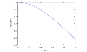
Auslenkung w(x) - ... für ϕ(ξ):
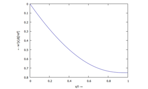
Querschnitts-Kippung w'(x) - ... für M(ξ):
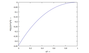
Momentenverlauf M(x) - ... für Q(ξ):
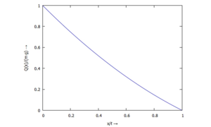
Querkraftverlauf Q(x)


/******************************************************/
/* post-processing                                    */

/* bearing forces and moments */
reactForces: [M[A] = M[ref]*M(0),
              Q[z] = Q[ref]*Q(0)];
reactForces: ratsimp(subst(sol, subst(subst([xi=0],displ),subst(reference,reactForces))));

/* plot displacements */

fcts: [ w (xi),
        ϕ (xi),
        M (xi),
        Q (xi)];

textlabels : ["← w(x)/w[rez]", "← w'(x)/ϕ[ref]", "M(x)/(m*g*ℓ) →", "Q(x)/(m g) →"];

for i: 1 thru 4 do(
  f : ratsimp(subst(geometry,subst(sol, subst(geometry,subst(dimless,subst(displ,subst(params,fcts[i]))))))),
  preamble: if i<=2 then "set yrange [] reverse" else "set yrange []",
  plot2d(f, [xi,0,1], [legend, false],
                      [gnuplot_preamble, preamble],
                      [xlabel, "x/ℓ →"],
                      [ylabel, textlabels[i]]) )$

/******************************************************/
/* print tabular values                                             */

for i: 1 thru 4 do(
  f : ratsimp(subst(geometry,subst(sol, subst(geometry,subst(dimless,subst(displ,subst(params,fcts[i])))))*facts[i])),
  N :100,
  print("table for",textlabels[i]),
  for j: 0 thru N do (
    t : j/N,
    print(float(t),";",expand(float(subst([xi=t],f))))
      ))$
Plot Data
Datenpunkte der Auslenkung w(ξ)
Die Tabelle enthält die Werte ξ und w(ξ) zum Herunterladen.

toggle: data listing →
table for ← w(x)/w[rez]
0.0 ; 0.0
0.01 ; 7.481203031248985*10^-5
0.02 ; 2.984924700020887*10^-4
0.03 ; 6.698993034749879*10^-4
0.04 ; 0.001187879040283986
0.05 ; 0.00185126660292937
0.06 ; 0.002658885214942354
0.07 ; 0.003609546289359847
0.08 ; 0.004702049317703514
0.09 ; 0.005935181759589655
0.1 ; 0.007307718933097404
0.11 ; 0.008818423906038287
0.12 ; 0.01046604738827592
0.13 ; 0.01224932762526032
0.14 ; 0.01416699029293324
0.15 ; 0.01621774839421548
0.16 ; 0.01840030215723649
0.17 ; 0.02071333893554073
0.18 ; 0.02315553311047674
0.19 ; 0.02572554599601331
0.2 ; 0.02842202574623001
0.21 ; 0.03124360726574977
0.22 ; 0.03418891212340282
0.23 ; 0.0372565484694203
0.24 ; 0.04044511095649053
0.25 ; 0.04375318066501066
0.26 ; 0.04717932503291399
0.27 ; 0.05072209779045508
0.28 ; 0.0543800389003753
0.29 ; 0.05815167450388911
0.3 ; 0.06203551687296655
0.31 ; 0.06603006436941357
0.32 ; 0.07013380141128575
0.33 ; 0.07434519844720817
0.34 ; 0.07866271193920962
0.35 ; 0.08308478435471277
0.36 ; 0.08760984416838222
0.37 ; 0.09223630587454254
0.38 ; 0.09696257001097904
0.39 ; 0.1017870231949183
0.4 ; 0.1067080381721125
0.41 ; 0.1117239738799426
0.42 ; 0.1168331755255615
0.43 ; 0.1220339746801493
0.44 ; 0.1273246893904267
0.45 ; 0.1327036243086318
0.46 ; 0.1381690708422802
0.47 ; 0.1437193073250795
0.48 ; 0.1493525992104727
0.49 ; 0.1550671992894059
0.5 ; 0.160861347933972
0.51 ; 0.1667332733687484
0.52 ; 0.1726811919717323
0.53 ; 0.1787033086069086
0.54 ; 0.1847978169906433
0.55 ; 0.1909629000942185
0.56 ; 0.1971967305850093
0.57 ; 0.2034974713089322
0.58 ; 0.2098632758170441
0.59 ; 0.2162922889392689
0.6 ; 0.2227826474085497
0.61 ; 0.229332480538859
0.62 ; 0.2359399109607717
0.63 ; 0.2426030554186048
0.64 ; 0.2493200256333157
0.65 ; 0.2560889292357581
0.66 ; 0.2629078707751271
0.67 ; 0.2697749528078152
0.68 ; 0.2766882770722823
0.69 ; 0.2836459457558966
0.7 ; 0.2906460628602184
0.71 ; 0.2976867356715562
0.72 ; 0.3047660763442248
0.73 ; 0.3118822036044391
0.74 ; 0.3190332445833526
0.75 ; 0.3262173367883804
0.76 ; 0.3334326302226785
0.77 ; 0.340677289663329
0.78 ; 0.3479494971096025
0.79 ; 0.3552474544135462
0.8 ; 0.3625693861060849
0.81 ; 0.3699135424327804
0.82 ; 0.3772782026145832
0.83 ; 0.3846616783500371
0.84 ; 0.392062317576676
0.85 ; 0.3994785085108331
0.86 ; 0.4069086839865492
0.87 ; 0.4143513261159026
0.88 ; 0.4218049712949479
0.89 ; 0.4292682155813812
0.9 ; 0.4367397204721419
0.91 ; 0.4442182191116147
0.92 ; 0.4517025229634247
0.93 ; 0.4591915289818366
0.94 ; 0.4666842273215563
0.95 ; 0.4741797096282359
0.96 ; 0.4816771779554077
0.97 ; 0.4891759543576916
0.98 ; 0.4966754912143446
0.99 ; 0.5041753823419752
1.0 ; 0.5116753749604923
Datenpunkte des Querschnitt-Kippwinkels ϕ(ξ)
Die Tabelle enthält die Werte ξ und ϕ(ξ) zum Herunterladen.
toggle: data listing →
table for ← w'(x)/ϕ[ref]
0.0 ; 0.0
0.01 ; 0.01494356203126184
0.02 ; 0.02977349250076523
0.03 ; 0.04448864954005514
0.04 ; 0.05908788004997918
0.05 ; 0.07357001972386588
0.06 ; 0.08793389308109258
0.07 ; 0.1021783135117721
0.08 ; 0.1163020833333333
0.09 ; 0.1303039938598174
0.1 ; 0.1441828254847645
0.11 ; 0.1579373477786176
0.12 ; 0.1715663196016297
0.13 ; 0.185068489233321
0.14 ; 0.1984425945195976
0.15 ; 0.2116873630387144
0.16 ; 0.2248015122873346
0.17 ; 0.2377837498880229
0.18 ; 0.250632773819587
0.19 ; 0.2633472726717744
0.2 ; 0.2759259259259259
0.21 ; 0.2883674042632877
0.22 ; 0.3006703699027901
0.23 ; 0.3128334769702193
0.24 ; 0.3248553719008265
0.25 ; 0.336734693877551
0.26 ; 0.348470075307174
0.27 ; 0.3600601423368639
0.28 ; 0.3715035154137372
0.29 ; 0.3827988098902226
0.3 ; 0.3939446366782007
0.31 ; 0.4049396029550786
0.32 ; 0.4157823129251701
0.33 ; 0.4264713686399656
0.34 ; 0.4370053708811148
0.35 ; 0.4473829201101928
0.36 ; 0.4576026174895895
0.37 ; 0.4676630659791486
0.38 ; 0.4775628715134888
0.39 ; 0.4873006442652675
0.4 ; 0.496875
0.41 ; 0.5062845615284206
0.42 ; 0.5155279602627784
0.43 ; 0.5246038378838899
0.44 ; 0.5335108481262327
0.45 ; 0.5422476586888658
0.46 ; 0.5508129532804857
0.47 ; 0.55920543380751
0.48 ; 0.5674238227146814
0.49 ; 0.5754668654883558
0.5 ; 0.5833333333333334
0.51 ; 0.5910220260348633
0.52 ; 0.5985317750182615
0.53 ; 0.6058614466194641
0.54 ; 0.6130099455807844
0.55 ; 0.6199762187871581
0.56 ; 0.6267592592592592
0.57 ; 0.6333581104210475
0.58 ; 0.6397718706605832
0.59 ; 0.6459996982043157
0.6 ; 0.6520408163265307
0.61 ; 0.6578945189172403
0.62 ; 0.6635601764335224
0.63 ; 0.6690372422611753
0.64 ; 0.674325259515571
0.65 ; 0.6794238683127573
0.66 ; 0.6843328135442192
0.67 ; 0.6890519531912488
0.68 ; 0.6935812672176308
0.69 ; 0.6979208670823379
0.7 ; 0.7020710059171598
0.71 ; 0.7060320894177032
0.72 ; 0.7098046875
0.73 ; 0.7133895467790936
0.74 ; 0.716787603930461
0.75 ; 0.72
0.76 ; 0.7230280957336108
0.77 ; 0.7258734880031728
0.78 ; 0.728538027411986
0.79 ; 0.7310238371695923
0.8 ; 0.7333333333333333
0.81 ; 0.7354692465221383
0.82 ; 0.7374346452168917
0.83 ; 0.7392329607714223
0.84 ; 0.7408680142687277
0.85 ; 0.7423440453686201
0.86 ; 0.7436657433056325
0.87 ; 0.7448382802098833
0.88 ; 0.7458673469387755
0.89 ; 0.7467591916240565
0.9 ; 0.7475206611570248
0.91 ; 0.748159245854726
0.92 ; 0.7486831275720165
0.93 ; 0.7491012315486069
0.94 ; 0.7494232823068707
0.95 ; 0.7496598639455783
0.96 ; 0.7498224852071006
0.97 ; 0.7499236497313602
0.98 ; 0.7499769319492503
0.99 ; 0.7499970591118518
1.0 ; 0.75
Datenpunkte des Biegemoments M(ξ)
Die Tabelle enthält die Werte ξ und M(ξ) zum Herunterladen.
toggle: data listing →
table for M(x)/(m*g*ℓ) ->
0.0 ; -0.4444444444444444
0.01 ; -0.434511
0.02 ; -0.4247102222222222
0.03 ; -0.4150414444444445
0.04 ; -0.405504
0.05 ; -0.3960972222222222
0.06 ; -0.3868204444444445
0.07 ; -0.377673
0.08 ; -0.3686542222222222
0.09 ; -0.3597634444444445
0.1 ; -0.351
0.11 ; -0.3423632222222222
0.12 ; -0.3338524444444445
0.13 ; -0.325467
0.14 ; -0.3172062222222222
0.15 ; -0.3090694444444445
0.16 ; -0.301056
0.17 ; -0.2931652222222222
0.18 ; -0.2853964444444445
0.19 ; -0.277749
0.2 ; -0.2702222222222222
0.21 ; -0.2628154444444444
0.22 ; -0.255528
0.23 ; -0.2483592222222222
0.24 ; -0.2413084444444444
0.25 ; -0.234375
0.26 ; -0.2275582222222222
0.27 ; -0.2208574444444444
0.28 ; -0.214272
0.29 ; -0.2078012222222222
0.3 ; -0.2014444444444445
0.31 ; -0.195201
0.32 ; -0.1890702222222222
0.33 ; -0.1830514444444444
0.34 ; -0.177144
0.35 ; -0.1713472222222222
0.36 ; -0.1656604444444444
0.37 ; -0.160083
0.38 ; -0.1546142222222222
0.39 ; -0.1492534444444444
0.4 ; -0.144
0.41 ; -0.1388532222222222
0.42 ; -0.1338124444444445
0.43 ; -0.128877
0.44 ; -0.1240462222222222
0.45 ; -0.1193194444444445
0.46 ; -0.114696
0.47 ; -0.1101752222222222
0.48 ; -0.1057564444444444
0.49 ; -0.101439
0.5 ; -0.09722222222222222
0.51 ; -0.09310544444444445
0.52 ; -0.089088
0.53 ; -0.08516922222222222
0.54 ; -0.08134844444444445
0.55 ; -0.077625
0.56 ; -0.07399822222222223
0.57 ; -0.07046744444444444
0.58 ; -0.067032
0.59 ; -0.06369122222222222
0.6 ; -0.06044444444444445
0.61 ; -0.057291
0.62 ; -0.05423022222222222
0.63 ; -0.05126144444444444
0.64 ; -0.048384
0.65 ; -0.04559722222222222
0.66 ; -0.04290044444444444
0.67 ; -0.040293
0.68 ; -0.03777422222222222
0.69 ; -0.03534344444444444
0.7 ; -0.033
0.71 ; -0.03074322222222222
0.72 ; -0.02857244444444445
0.73 ; -0.026487
0.74 ; -0.02448622222222222
0.75 ; -0.02256944444444444
0.76 ; -0.020736
0.77 ; -0.01898522222222222
0.78 ; -0.01731644444444444
0.79 ; -0.015729
0.8 ; -0.01422222222222222
0.81 ; -0.01279544444444444
0.82 ; -0.011448
0.83 ; -0.01017922222222222
0.84 ; -0.008988444444444445
0.85 ; -0.007875
0.86 ; -0.006838222222222222
0.87 ; -0.005877444444444445
0.88 ; -0.004992
0.89 ; -0.004181222222222222
0.9 ; -0.003444444444444444
0.91 ; -0.002781
0.92 ; -0.002190222222222222
0.93 ; -0.001671444444444444
0.94 ; -0.001224
0.95 ; -8.472222222222222*10^-4
0.96 ; -5.404444444444444*10^-4
0.97 ; -3.03*10^-4
0.98 ; -1.342222222222222*10^-4
0.99 ; -3.344444444444444*10^-5
1.0 ; 0.0
Datenpunkte der Querkraft Q(ξ)
Die Tabelle enthält die Werte ξ und Q(ξ) zum Herunterladen.
toggle: data listing →
table for Q(x)/(m g) ->
0.0 ; 1.0
0.01 ; 0.9867
0.02 ; 0.9734666666666667
0.03 ; 0.9603
0.04 ; 0.9472
0.05 ; 0.9341666666666667
0.06 ; 0.9212
0.07 ; 0.9083
0.08 ; 0.8954666666666666
0.09 ; 0.8827
0.1 ; 0.87
0.11 ; 0.8573666666666667
0.12 ; 0.8448
0.13 ; 0.8323
0.14 ; 0.8198666666666666
0.15 ; 0.8075
0.16 ; 0.7952
0.17 ; 0.7829666666666667
0.18 ; 0.7708
0.19 ; 0.7587
0.2 ; 0.7466666666666667
0.21 ; 0.7347
0.22 ; 0.7228
0.23 ; 0.7109666666666666
0.24 ; 0.6992
0.25 ; 0.6875
0.26 ; 0.6758666666666666
0.27 ; 0.6643
0.28 ; 0.6528
0.29 ; 0.6413666666666666
0.3 ; 0.63
0.31 ; 0.6187
0.32 ; 0.6074666666666667
0.33 ; 0.5963
0.34 ; 0.5852
0.35 ; 0.5741666666666667
0.36 ; 0.5632
0.37 ; 0.5523
0.38 ; 0.5414666666666667
0.39 ; 0.5307
0.4 ; 0.52
0.41 ; 0.5093666666666666
0.42 ; 0.4988
0.43 ; 0.4883
0.44 ; 0.4778666666666667
0.45 ; 0.4675
0.46 ; 0.4572
0.47 ; 0.4469666666666667
0.48 ; 0.4368
0.49 ; 0.4267
0.5 ; 0.4166666666666667
0.51 ; 0.4067
0.52 ; 0.3968
0.53 ; 0.3869666666666667
0.54 ; 0.3772
0.55 ; 0.3675
0.56 ; 0.3578666666666667
0.57 ; 0.3483
0.58 ; 0.3388
0.59 ; 0.3293666666666666
0.6 ; 0.32
0.61 ; 0.3107
0.62 ; 0.3014666666666667
0.63 ; 0.2923
0.64 ; 0.2832
0.65 ; 0.2741666666666667
0.66 ; 0.2652
0.67 ; 0.2563
0.68 ; 0.2474666666666667
0.69 ; 0.2387
0.7 ; 0.23
0.71 ; 0.2213666666666667
0.72 ; 0.2128
0.73 ; 0.2043
0.74 ; 0.1958666666666667
0.75 ; 0.1875
0.76 ; 0.1792
0.77 ; 0.1709666666666667
0.78 ; 0.1628
0.79 ; 0.1547
0.8 ; 0.1466666666666667
0.81 ; 0.1387
0.82 ; 0.1308
0.83 ; 0.1229666666666667
0.84 ; 0.1152
0.85 ; 0.1075
0.86 ; 0.09986666666666667
0.87 ; 0.0923
0.88 ; 0.0848
0.89 ; 0.07736666666666667
0.9 ; 0.07
0.91 ; 0.0627
0.92 ; 0.05546666666666666
0.93 ; 0.0483
0.94 ; 0.0412
0.95 ; 0.03416666666666666
0.96 ; 0.0272
0.97 ; 0.0203
0.98 ; 0.01346666666666667
0.99 ; 0.0067
1.0 ; 0.0
Links
Literature
- ...