Gelöste Aufgaben/JUMP/E-Motor and Drive-Train: Unterschied zwischen den Versionen
| (41 dazwischenliegende Versionen desselben Benutzers werden nicht angezeigt) | |||
| Zeile 22: | Zeile 22: | ||
Losses in the DC/DC converter shall be small - so for input port “1“ and output port “2“ we obtain | Losses in the DC/DC converter shall be small - so for input port “1“ and output port “2“ we obtain | ||
::<math> | ::<math>U_B \cdot I_B = U_M \cdot I_M</math> . | ||
Let the “gas”-pedal-indicator “''p''“ control | Let the “gas”-pedal-indicator “''p''“ control | ||
::<math> | ::<math>U_M = p \cdot U_B \text{; } 0 \le p \le 1.</math> | ||
with | with | ||
| Zeile 40: | Zeile 40: | ||
::<math>\omega_M \cdot M_M = \omega_W \cdot M_W</math>. | ::<math>\omega_M \cdot M_M = \omega_W \cdot M_W</math>. | ||
Fortunately, this relationship is already "hardwired" in the [[Werkzeuge/Gleichgewichtsbedingungen/Arbeitsprinzipe der Analytischen Mechanik/Prinzip der virtuellen Verrückungen|Principle of Virtual Work]]. | |||
And we have only one differential equation for the electrical components: | And we have only one differential equation for the electrical components: | ||
| Zeile 56: | Zeile 57: | ||
with ''U<sub>R</sub>, U<sub>L</sub>'' being the differential voltage over resistance ''R'' and inductance ''L'' respectively. “''e''” is the back electromagnetic force with | with ''U<sub>R</sub>, U<sub>L</sub>'' being the differential voltage over resistance ''R'' and inductance ''L'' respectively. “''e''” is the back electromagnetic force with | ||
::<math>e = k_e\cdot \ | ::<math>e = k_e\cdot \tilde{\omega}_M</math> | ||
and the electromotive force constant ''k<sub>e</sub>''. Note the | and the electromotive force constant ''k<sub>e</sub>''. Note the <math>\tilde{\omega}_M</math> is the differential rotational velocity between rotor and stator, i.e. | ||
::<math>\ | ::<math>\tilde{\omega}_M = \dot{\psi}_M(t) - \dot{\phi}(t).</math> | ||
Employing | Employing | ||
| Zeile 68: | Zeile 69: | ||
and using | and using | ||
::<math>M_M = | ::<math>M_M = k_T \cdot I_M</math> | ||
with the armature constant ''k<sub> | with the armature constant ''k<sub>T</sub>'', we have the complete set of equations. | ||
From the above, we find | From the above, we find | ||
| Zeile 135: | Zeile 136: | ||
Since the gearbox is built into the car, the wheel-side relative gear-box-angle is | Since the gearbox is built into the car, the wheel-side relative gear-box-angle is | ||
::<math>\tilde{\psi}_{W} = \psi_W(t) | ::<math>\tilde{\psi}_{W} = \psi_W(t) + \phi(t)</math> | ||
and on the motor-side | and on the motor-side | ||
::<math>\tilde{\psi}_{M} = \psi_M(t) | ::<math>\tilde{\psi}_{M} = \psi_M(t) - \phi(t)</math>. | ||
With the gear transmission ratio | With the gear transmission ratio | ||
| Zeile 235: | Zeile 236: | ||
and with this algebraic equation | and with this algebraic equation | ||
::<math>e = k_e \cdot \left(\dot{\psi} | ::<math>e = k_e \cdot \underbrace{\left(\dot{\psi}_M(t) + \dot{\phi}(t) \right)}_{\displaystyle =\tilde{\omega}_M = n_G \cdot \tilde{\omega}_W}</math>. | ||
Keep in mind that <math>\tilde{\omega}_M</math> and <math>\tilde{\omega}_W</math> are the rotational velocities of the gearbox-shafts '''relative''' to the car-body, thus | |||
::<math>\begin{array}{ll}\tilde{\omega}_W &= \frac{\displaystyle d\,\tilde{\psi}}{\displaystyle d\, t}\\ | |||
&= \left( \underbrace{\frac{\displaystyle d\, \psi}{\displaystyle d\, t}}_{\displaystyle =\omega} - \frac{\displaystyle d\, \phi}{\displaystyle d\, t}\right)\end{array}</math>. | |||
==Variables== | ==Variables== | ||
| Zeile 250: | Zeile 256: | ||
==Parameter== | ==Parameter== | ||
System parameters for the motor are ''k<sub>T</sub> | System parameters for the motor are ''k<sub>T</sub>, k<sub>e</sub>'' and ''R<sub>M</sub>'' . For the stationary (<math>\frac{\displaystyle d \; I_M}{\displaystyle dt} = 0</math>) - condition, we derive | ||
::<math>M_M=\frac{{U_M}\, {k_T}-{k_T}\, {k_e} \ | ::<math>M_M=\frac{{U_M}\, {k_T}-{k_T}\, {k_e} \tilde{\omega}_M }{{R_M}}</math>. | ||
For our application, it will be easier to replace ''k<sub>e</sub>'', ''k<sub>R</sub>'' and ''R'' by mechanical properties as | |||
<ol> | |||
<li>under a "no-load"-condition ''M<sub>M</sub>=0'', we have | |||
::<math>\ | ::<math>k_e= \frac{U_M}{\tilde{\omega}_{NL}}</math></li> | ||
<li>under the "stalled motor"-condition <math>\tilde{\omega}_{St}=0</math>, we have | |||
::<math>M_{St} = \frac{ | ::<math>k_T = \frac{\displaystyle M_{St}}{\displaystyle I_{St}}</math> and <math>R = \frac{\displaystyle U_M}{\displaystyle I_{St}}</math>.</li> | ||
</ol> | |||
Thus | Thus for ''U<sub>M</sub> = 12 V'' we can import measured performance parameters and then replace ''k<sub>T</sub>, k<sub>e</sub>'' and ''R<sub>M</sub>'' by <math>\tilde{\omega}_{NL}</math> | ||
{| class="wikitable" | ''I<sub>St</sub>'' and ''M<sub>St</sub>''. | ||
!name | |||
{| class="wikitable" style="border-collapse: collapse;" | |||
!style="border-right: solid 0px;"|name | |||
!symbol | !symbol | ||
!value | !value | ||
!unit | !unit | ||
|- | |||
|nominal voltage | |||
|''U<sub>ref</sub>'' | |||
|12 | |||
|V | |||
|- | |- | ||
|no-load rotational speed | |no-load rotational speed | ||
|'' | |<math>\tilde{\omega}_{NL}</math> | ||
| | |14800 | ||
| | |rpm | ||
|- | |||
|stall-current | |||
|''I<sub>St</sub>'' | |||
|8.6 | |||
|A | |||
|- | |- | ||
|stall-torque | |stall-torque | ||
| Zeile 287: | Zeile 307: | ||
|gear tramission ratio | |gear tramission ratio | ||
|''n<sub>G</sub>'' | |''n<sub>G</sub>'' | ||
| | |25 | ||
|1 | |1 | ||
|} | |} | ||
[[Gelöste Aufgaben/JUMP|Back to Start →]] | [[Gelöste Aufgaben/JUMP|Back to Start →]] | ||
Aktuelle Version vom 24. März 2021, 15:54 Uhr
Scope

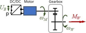
The Drive-Train consists of a DC/DC-converter, a DC Motor and a gear-box.
- DC/DC-converter: is supplied with the battery voltage UB, the output voltage is controlled by the driver via setpoint “p“.
- motor: is a standard DC brushed motor, the manufacturer provides only few information on its characteristics - we’ll need to improvise.
- gearbox: has a gear ratio of ratio of nG=100, its shaft rotates at speed ωW and delivers a torque MW to the front wheels.
The task is: provide a mathematical model for the drive train that accounts for load-alterations imposed by the driver. And we assume losses in the two converters - DC/DC and gearbox - to be negligible.
Structure

The drive train receives a "gas"-pedal position "p" from the driver and a battery-voltage UB.
It delivers a torque MW on the wheel and creates an electric current IM through the motor.

The sub-model consists of DC/DC-converter, Motor and gear-box:
DC/DC Converter
Losses in the DC/DC converter shall be small - so for input port “1“ and output port “2“ we obtain
- .
Let the “gas”-pedal-indicator “p“ control
with
Motor

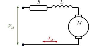
We use a common electric circuit representation for a series wound motor, the field coils are connected electrically in series with the armature coils, resistance R sums up all electrical losses in the motor.
Gearbox
Losses in the gearbox shall be small - so for input (ωM, MM) and output (ωW, MW) we obtain the fixed relation
- .
Fortunately, this relationship is already "hardwired" in the Principle of Virtual Work. And we have only one differential equation for the electrical components:
- ,
the remaining equations are algebraic.
Model
Electrical Components
For the motor, we find with Kirchhoff's law that
with UR, UL being the differential voltage over resistance R and inductance L respectively. “e” is the back electromagnetic force with
and the electromotive force constant ke. Note the is the differential rotational velocity between rotor and stator, i.e.
Employing
and using
with the armature constant kT, we have the complete set of equations.
From the above, we find
and additionally the algebraic equations
- .
/*******************************************************/
/* MAXIMA script                                       */
/* version: wxMaxima 16.04.2                           */
/* author: Andreas Baumgart                            */
/* last updated: 2021-02-08                            */
/* ref: Modelling and Simulation (TUAS)                */
/* description: virtual work of drive train electrics  */
/*******************************************************/

/*******************************************************/
/* declarations                                        */
/*******************************************************/
declare("φ", alphabetic);
declare("ψ", alphabetic);
declare("ω", alphabetic);

/*******************************************************/
/* kinematics                                          */
/*******************************************************/
kirchhoff : [U[M] = p(t)*U[B],
	     U[B]*I[B] = U[M]*I[M],
	     U[M] = U[R] + U[L] + e,
             e = k[e]*omega[M],
	     ω[M] = diff(ψ[M](t),t)+diff(φ(t),t),
	     U[R] = R*I[M](t),
	     U[L] = L * diff(I[M](t),t),
	     M[M] = k[t]*I[M](t)];

solve(kirchhoff[7], [diff(I[M](t),t)]);
Mechanical Components
The Virtual Work of d'Alembert forces, motor torque MM and wheel torque MW is
- .
Since the gearbox is built into the car, the wheel-side relative gear-box-angle is
and on the motor-side
- .
With the gear transmission ratio
and
we find
with
- .
We have thus "returned" all state variables to the Car-Body-submodel.
/*******************************************************/
/* MAXIMA script                                       */
/* version: wxMaxima 16.04.2                           */
/* author: Andreas Baumgart                            */
/* last updated: 2021-02-08                            */
/* ref: Modelling and Simulation (TUAS)                */
/* description: virtual work of drive train mechanics  */
/*******************************************************/

/*******************************************************/
/* declarations                                        */
/*******************************************************/
declare("δ", alphabetic);
declare("φ", alphabetic);
declare("ψ", alphabetic);

/*******************************************************/
/* kinematics                                          */
/*******************************************************/
kin : [ψ[M,r] = n[G]*ψ[W,r],
       ψ[W,r] = ψ[W](t) - φ(t),
       ψ[M,r] = ψ[M](t) + φ(t)];
Q : [ψ[M](t),ψ[M,r],ψ[W,r]];
sol: ratsimp(solve(kin,Q))[1];


/* Principle of Virtual Work */
PVW: δW = - J[M]*diff(ψ[M](t),t,2)*δψ[M] + M[M]*(δψ[M]+δφ) - M[W]*δψ[W];

/* minimal coordinates */
q : [ φ(t), ψ[W](t)];
δq: [δφ   ,δψ[W]   ];

varia: [ψ[M](t)=δψ[M],ψ[M,r]=δψ[M,r],ψ[W,r]=δψ[W,r],
        ψ[W](t)=δψ[W], φ(t) =δφ];
sol : expand(append(sol, subst(varia,sol)));

PVW : expand(subst(sol,PVW));
PVW : ev(PVW,nouns);

eom : makelist(coeff(rhs(PVW),δq[i]),i,1,2);
eom : ratsimp(eom);

MM : funmake('matrix,makelist(makelist(ratsimp(coeff(-eom[i],'diff(q[j],t,2))),j,1,2),i,1,2));

rest : expand(eom + makelist(sum(MM[i,j]*diff(q[j],t,2),j,1,2),i,1,2));

print(δq, "*(-",MM,"*",transpose(diff(q,t,2)),"+",transpose(rest),") = 0")$
Consequently, the drive train has only one state-variable: IM:
where
and with this algebraic equation
- .
Keep in mind that and are the rotational velocities of the gearbox-shafts relative to the car-body, thus
- .
Variables
| name | symbol | unit |
|---|---|---|
| motor current | IM | A |
Parameter
System parameters for the motor are kT, ke and RM . For the stationary () - condition, we derive
- .
For our application, it will be easier to replace ke, kR and R by mechanical properties as
- under a "no-load"-condition MM=0, we have
- under the "stalled motor"-condition , we have
- and .
Thus for UM = 12 V we can import measured performance parameters and then replace kT, ke and RM by ISt and MSt.
| name | symbol | value | unit |
|---|---|---|---|
| nominal voltage | Uref | 12 | V |
| no-load rotational speed | 14800 | rpm | |
| stall-current | ISt | 8.6 | A |
| stall-torque | MSt | 0.042 | N m |
| inductance | L | 0.05 | H |
| gear tramission ratio | nG | 25 | 1 |
References
- ...