Gelöste Aufgaben/JUMP/Car-Body

← Back to Start

Scope

Car-Body

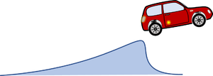
In common simulation applications - especially for full-size commercial cars - the pitch-angle of the car is assumed to be small to allow for a linearization of geometry and most parts of the equations of motion. We drop this limitation so we can do more fancy stuff with our model - like climbing steep roads or jumping across ditches.

Block Diagram.

We employ a spatial x-y coordinate system, x in horizontal, y in vertical, upwards direction. And we’ll briefly employ the z-axis as rotation direction - which is towards you following the “right-hand-rule“ for coordinate systems.

Structure

The driver controls the car's motion via the position of the "gas"-pedal, which is being translated into a torque M_W at the wheel.

This toque will change velocities and thus the position of the car. These state-variables will then create - via info - a feedback to the driver.

We’ll need to invest significant efforts in describing the kinematics of the car-motion and to derive its equations of body-motion since we do not want to limit our study on small pitch-angles of the car. Key accessory will be vectors, which map locations like the center of mass:

${\vec {r}}_{C}(t)$.

This vector has - in 2D - two coordinates $u_{1}(t),u_{2}(t)$, measured in the inertial x-y frame:

${\vec {r}}_{C}(t)={\vec {\underline {e}}}_{0}\cdot \left({\begin{array}{c}u_{1}\\u_{2}\end{array}}\right)$ with ${\vec {\underline {e}}}_{0}=\left({\vec {e}}_{x},{\vec {e}}_{y}\right)$.

representing the unit vectors spanning the x-y space. If we refer to a specific frame, we may drop the vector-notation $({\vec {.}})$ and refer to the column-matrix of coordinates $({\underline {.}})$ only, so

${\underline {r}}_{C}=\left({\begin{array}{c}u_{1}\\u_{2}\end{array}}\right)$.

We’ll also employ coordinate transformations using Euler-rotations.

The car with front-wheel drive consists of the car-body with center of mass “C“, the front wheels “A“ and the rear wheel “B“. Masses of car-body and wheel-sets are M and m respectively.The geometry of the car is described by

• a₀: the wheel base;
• a₁: longitudinal distance between center of mass and front-wheel-hub;
• a₂ = a₀ - a₁ and
• a₃: vertical distance between center of mass and front-wheel-hub (relaxed springs).

Body

We use five coordinates to describe the motion of the car:

• $u_{1}(t),u_{2}(t),\varphi (t)$ for the location of the center of mass of the car-body and its pitch-angle
  ,
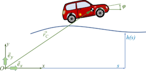• $u_{3},u_{4}$ for the "vertical" motion of the wheel hubs relative to the car-body - which is synonym to the compression of the springs
  
  and
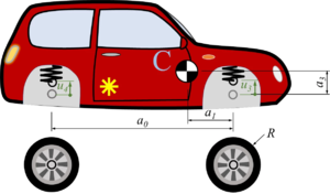
• $\psi (t)$ as the rotation angle of the front-wheel - we'll not account for the rotation of the rear-wheel.

So the center of mass of the car-body is

${\vec {r}}_{M}={\vec {\underline {e}}}_{0}\cdot \left({\begin{array}{c}u_{1}(t)\\u_{2}(t)\end{array}}\right)$,

the coordinate system of the car is

${\vec {\underline {e}}}_{C}={\vec {\underline {e}}}_{0}\cdot {\underline {\underline {D}}}(\varphi (t))$

where

${\underline {\underline {D}}}(\varphi )=\left({\begin{array}{rr}\cos(\varphi )&-\sin(\varphi )\\+\sin(\varphi )&\cos(\varphi )\\\end{array}}\right)$.

So the location of the front-wheel “A“ is

${\vec {r}}_{A}={\vec {r}}_{M}+{\vec {r}}_{MA}$

or

${\underline {r}}_{A}={\underline {r}}_{M}+{\underline {\underline {D}}}(\varphi (t))\cdot \left({\begin{array}{c}a_{1}\\-a_{3}+u_{3}(t)\end{array}}\right)$.

Likewise, the location of the rear-wheel “B“ is

${\underline {r}}_{B}={\underline {r}}_{M}+{\underline {\underline {D}}}(\varphi (t))\cdot \left({\begin{array}{c}-a_{2}\\-a_{3}+u_{4}(t)\end{array}}\right)$

and in the following, we’ll be using the abbreviations

$\left({\begin{array}{c}U_{3}\\U_{4}\end{array}}\right)=:{\underline {r}}_{A}$

and

$\left({\begin{array}{c}U_{5}\\U_{6}\end{array}}\right)=:{\underline {r}}_{B}$.

Track

Tack specification

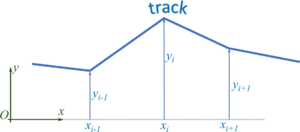
We describe the road by road-sections, which we call tracks. We start by defining each track as a line-segment, i.e. a first-order polynomial. The road is thus defined by pairs of track-endpoints, i.e. (x_i, y_i).

The track-polynomials are

${\begin{array}{ll}t_{i}(x)&=y_{i}\cdot {\tilde {x}}_{i}+y_{i-1}\cdot \left(1-{\tilde {x}}_{i}\right){\text{ for }}{\tilde {x}}_{i}={\frac {\displaystyle x-x_{i-1}}{\displaystyle x_{i}-x_{i-1}}}\\&=T_{i,1}\cdot x+T_{i,0}\end{array}}$.

During the numerical integration of the initial-value-problem - when the car runs along the track - the solver needs to cope with the transition between two straight lines - which is numerically more efficient if we convert the road in a continuously differentiable function.

Rounding the edges.

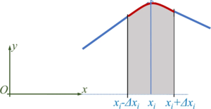
For this purpose, we define transition polynomials p_i of second degree - parabolas - as

$p_{i}(x)=\displaystyle \sum _{j=0}^{2}P_{i,j}\cdot x^{j}$

which connect two neighboring tracks.

The boundary conditions for the parabolas (red) and the neighboring lines (blue) yield

${\begin{array}{ll}\color {blue}t_{i}(x_{i}-\Delta x_{i})&=\color {red}p_{i}(x_{i}-\Delta x_{i}),\\\color {blue}\left.{\frac {\displaystyle dt_{i}}{\displaystyle dx_{i}}}\right\vert _{x_{i}-\Delta x_{i}}&=\color {red}\left.{\frac {\displaystyle dp_{i}}{\displaystyle dx_{i}}}\right\vert _{x_{i}-\Delta x_{i}},\\\color {blue}t_{i+1}(x_{i}+\Delta x_{i})&=\color {red}p_{i}(x_{i}+\Delta x_{i}),\\\color {blue}\left.{\frac {\displaystyle dt_{i+1}}{\displaystyle dx_{i+1}}}\right\vert _{x_{i}+\Delta x_{i}}&=\color {red}\left.{\frac {\displaystyle dp_{i}}{\displaystyle dx_{i}}}\right\vert _{x_{i}+\Delta x_{i}}.\end{array}}$

And though we have four boundary conditions, they allow for a solution with three unknown polynomial coefficients P_i if Δx_i is identical left and right from x_i - which we have already implied.

${\begin{array}{ll}{b_{3}}&=0,\\{b_{2}}&={\frac {\displaystyle {a_{2,1}}-{a_{1,1}}}{\displaystyle 4{\mathit {\Delta x_{i}}}}},\\{b_{1}}&={\frac {\displaystyle \left({a_{2,1}}+{a_{1,1}}\right)\,{\mathit {\Delta x_{i}}}-{x_{i}}\,{a_{2,1}}+{x_{i}}\,{a_{1,1}}}{\displaystyle 2{\mathit {\Delta x_{i}}}}},\\{b_{0}}&={\frac {\displaystyle \left({a_{2,1}}-{a_{1,1}}\right)\,{{\mathit {\Delta x_{i}}}^{2}}+\left(-2{x_{i}}\,{a_{2,1}}-2{x_{1}}\,{a_{1,1}}+4{y_{i}}\right)\,{\mathit {\Delta x_{i}}}+{{x}_{i}^{2}}\,{a_{2,1}}-{{x}_{i}^{2}}\,{a_{1,1}}}{\displaystyle 4{\mathit {\Delta x_{i}}}}}\end{array}}$

and

${\begin{array}{ll}{a_{1,0}}&={y_{i}}-{x_{i}}\,{a_{1,1}},\\{a_{1,1}}&={\frac {\displaystyle {y_{i-1}}-{y_{i}}}{\displaystyle {x_{i-1}}-{x_{i}}}}\operatorname {,} \\{a_{2,0}}&={y_{i}}-{x_{i}}\,{a_{2,1}},\\{a_{2,1}}&={\frac {\displaystyle {y_{i}}-{y_{i+1}}}{\displaystyle {x_{i}}-{x_{i+1}}}}\end{array}}$

But instead of employing the above, we solve the linear systems of equations for the coefficients numerically.

Now each polynomial creates new endpoints x_i - Δx_i and x_i + Δx_i which substitute for the initial x_i-point. The tracks are represented by a succession of lines and parabolas.

Next we need to find the contact point between wheel and road!

/*******************************************************/
/* MAXIMA script                                       */
/* version: wxMaxima 16.04.2                           */
/* author: Andreas Baumgart                            */
/* last updated: 2021-02-08                            */
/* ref: Modelling and Simulation (TUAS)                */
/* description: Rounding between straight line-segments*/
/*******************************************************/

/*******************************************************/
/* declarations                                        */
/*******************************************************/
declare("Δ",alphabetic);

params: [x[0] = 0, x[1] = 10, x[2]=15,
         y[0] = 0, y[1] =  1, y[2]=-1,
	 eps = 0.2];

/*******************************************************/
/* polynomials                                         */
/*******************************************************/
/* polynomial coefficiets of two consecutive straigt lines */
P : [[a[1,1],a[1,0]],[a[2,1],a[2,0]]];
/* polynomials of cubic and two consecutive linear polynomials */
p : [a[1,1]*x+a[1,0],
     b[3]*x^3+b[2]*x^2+b[1]*x+b[0],
     a[2,1]*x+a[2,0]];

/* compute polynomial coefficients from (x[i]/y[i])-points*/
linear : solve([subst([x=x[0]],p[1]) = y[0],
                subst([x=x[1]],p[1]) = y[1],
		subst([x=x[1]],p[3]) = y[1],
		subst([x=x[2]],p[3]) = y[2]], [a[1,0],a[1,1],a[2,0],a[2,1]])[1];
/* equations to continuously fit cubic function to lines */
equs : [subst([x=x[1]-Δx], p[1]) = subst([x=x[1]-Δx], p[2]),
        subst([x=x[1]+Δx], p[3]) = subst([x=x[1]+Δx], p[2]),
	subst([x=x[1]-Δx], diff(p[1],x)) = subst([x=x[1]-Δx], diff(p[2],x)),
	subst([x=x[1]+Δx], diff(p[3],x)) = subst([x=x[1]+Δx], diff(p[2],x))];
/* unknowns */
Q : [b[3],b[2],b[1],b[0]];

/* solve for unknowns */
sol : ratsimp(subst(linear,solve(equs,Q)[1]));

/* solve linear system of equations for unknown coefficients */
ACM : augcoefmatrix(equs,Q);
print(submatrix(ACM,5)," * ",transpose(Q)," = ",col(ACM,5))$


/* or - more simple when doing it numerically  .... */

/* coefficients of straigt line polynomials */
s : makelist(a[i,1] = (y[i-1]-y[i])/(x[i-1]-x[i]),i,1,2);

P : [[a[1,1],a[1,0]],[a[2,1],a[2,0]]];
p : [a[1,1]*x+a[1,0],
     b[3]*x^3+b[2]*x^2+b[1]*x+b[0],
     a[2,1]*x+a[2,0]];

linear : solve([subst([x=x[1]],p[1]) = y[1],
		subst([x=x[1]],p[3]) = y[1]], [a[1,0],a[2,0]])[1];

equs : [subst([x=x[1]-Δx], p[1]) = subst([x=x[1]-Δx], p[2]),
        subst([x=x[1]+Δx], p[3]) = subst([x=x[1]+Δx], p[2]),
	subst([x=x[1]-Δx], diff(p[1],x)) = subst([x=x[1]-Δx], diff(p[2],x)),
	subst([x=x[1]+Δx], diff(p[3],x)) = subst([x=x[1]+Δx], diff(p[2],x))];
Q : [b[3],b[2],b[1],b[0]];

sol : ratsimp(subst(linear,solve(equs,Q)))[1];

/* check with parameters */
subst(params,subst(s,subst(linear,solve(equs,Q))));

Contact-Point and -Normal

Contact conditions.

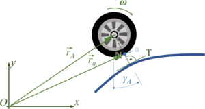
Finding the contact between wheel and road is our next challenge. We need to differentiate between the straight lines and the parabolas - but in both cases, we are looking for the equation of the normal “N“ to the road-surface, which cuts through the wheel-hub.

From the car-coordinates, we know the location of the wheel - e.g. “A” - expressed by its hub-vector

${\vec {r}}_{A}={\vec {\underline {e}}}_{0}\cdot \left({\begin{array}{c}U_{3}(t)\\U_{4}(t)\end{array}}\right)$.

And we can also define

${\vec {r}}_{A}(t)={\vec {r}}_{a}(t)+{\vec {N}}_{A}(t)$.

where ${\vec {r}}_{A}$ is the vector to the contact point “a“ of wheel “A“ and ${\vec {N}}_{A}$ is the vector from “a“ to the wheel hub “A“. Since "a" is a point on a track - if wheel and road have contact - and the direction of N_A is known to be perpendicular to this track in “a”, we have two equations for the two unknowns “point on track“ and “length of normal ${\vec {N}}_{A}$“.

Contact angles

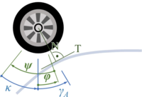
However, it remains tricky to find the material coordinate of the wheel that is at “a“. The picture below explains how first rotate the car by φ - positive about the z-axis, then rotate the wheel in negative direction by ψ and by κ in positive direction back to vertical. From there it is the known angle γ_A to “a“.

This succession of rotations is expressed by

$\gamma _{A}(t)=\varphi (t)-\psi (t)+\kappa (t)$

and we find contact point “a“ from

${\begin{array}{ll}{\underline {r}}_{a}&={\underline {r}}_{A}+{\underline {\underline {D}}}(\gamma _{A}(t))\cdot \left({\begin{array}{c}0\\-R\end{array}}\right)\\&={\begin{pmatrix}+R\sin {\left(\operatorname {\gamma } _{A}(t)\right)}-\left({u_{3}}(t)-{a_{3}}\right)\sin {\left(\operatorname {\varphi } (t)\right)}+{a_{1}}\cos {\left(\operatorname {\varphi } (t)\right)}+{u_{1}}(t)\\-R\cos {\left(\operatorname {\gamma } _{A}(t)\right)}+{a_{1}}\sin {\left(\operatorname {\varphi } (t)\right)}+\left({u_{3}}(t)-{a_{3}}\right)\cos {\left(\operatorname {\varphi } (t)\right)}+{u_{2}}(t)\end{pmatrix}}\end{array}}$

and “b“ from

${\begin{array}{ll}{\underline {r}}_{b}&={\underline {r}}_{B}+{\underline {\underline {D}}}(\gamma _{B}(t))\cdot \left({\begin{array}{c}0\\-R\end{array}}\right)\\&={\begin{pmatrix}+\sin {\left({\gamma _{B}}\right)}R-\left({u_{4}}(t)-{a_{3}}\right)\sin {\left(\operatorname {\varphi } (t)\right)}-{a_{2}}\cos {\left(\operatorname {\varphi } (t)\right)}+{u_{1}}(t)\\-\cos {\left({\gamma _{B}}\right)}R-{a_{2}}\sin {\left(\operatorname {\varphi } (t)\right)}+\left({u_{4}}(t)-{a_{3}}\right)\cos {\left(\operatorname {\varphi } (t)\right)}+{u_{2}}(t)\end{pmatrix}}\end{array}}$.

For wheel A und B, the angles ψ and κ are not identical - but we have dropped the indices here for brevity.

Track is a Line

If the track is line “i“, we have

${\vec {r}}_{a}={\vec {\underline {e}}}_{0}\cdot \left[\right.\underbrace {\left({\begin{array}{c}x_{i-1}\\y_{i-1}\end{array}}\right)} _{\displaystyle :={\underline {P}}_{i-1}}+\xi \cdot \underbrace {\left({\begin{array}{c}x_{i}-x_{i-1}\\y_{i}-y_{i-1}\end{array}}\right)} _{:=\displaystyle {\underline {\Delta P}}_{i}}\left.\right]$

with

${\underline {P}}_{i-1},{\underline {P}}_{i}$

being start- end end-points of the line with coordinates [x_i, h_i] and ξ naming the coordinate of point “C“. For the track-normal, we have

${\vec {N}}_{A}=\eta \cdot R\cdot {\vec {n}}_{A}$

with the unit-normal , the wheel-radius R and the unknown η. For the unit-normal

${\vec {N}}_{A}\cdot \Delta {\vec {P}}_{i}=0{\text{ and }}{\vec {n}}_{A}\cdot {\vec {n}}_{A}=1$

holds.

And for the contact angles γ_A/B we employ

$\tan \gamma _{A}(t)={\frac {\displaystyle N_{A,y}}{\displaystyle N_{A,x}}}$.

Track is a Parabola

If the track is defined by a second-order polynomial p_i, we proceed accordingly. However, the track inclination is linearly dependent on “x” and we find that the normal is proportional to:

${\underline {\tilde {N}}}=\left({\begin{array}{c}1\\-{\frac {\displaystyle 1}{\displaystyle 2\;P_{i,2}\;x+P_{i,1}}}\end{array}}\right).$

From

${\underline {r}}_{A}=\left({\begin{array}{c}x\\p_{i}(x)\end{array}}\right)+\eta \cdot {\underline {\tilde {N}}}{\text{ with }}{\underline {r}}_{A}=\left({\begin{array}{c}U_{3}\\U_{4}\end{array}}\right)$

we get two equations for the unknowns “x“ and “η“ as

${\begin{array}{ll}u_{3}&=\eta +x,\\u_{4}&=-{\frac {\displaystyle \eta }{\displaystyle 2P_{i,2}\;x+P_{i,1}}}+P_{i,2}\,{{x}^{2}}+P_{i,1}x+P_{i,0}\end{array}}$.

And we get a third-degree polynomial in “x“ from the second equation. The three solutions for point “C” usually comprise complex (they have a real and imaginary part) solutions depending on the curvature (convex or concave) of the parabola. That’s not a problem but increases computational cost significantly - because we will need to solve this equation for each value of U₃, U₄ again and again.

Contact Forces

Wheel kinematics

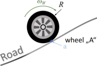
At contact “a” between road and wheel, the motor-torque must be transformed into a propulsion force of the car.

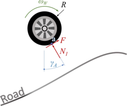
In the freebody-diagram for wheel “A“ below, we account for the contact forces

• normal force N_a and
• traction force F.

The interaction between road and wheel is a complex relationship between these two forces and the relative velocity v_rel of the wheel in point C relative to the road.

Contact forces F, N

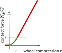
For the normal force N_A we assume a characteristic which depends on the dimensionless compression of the wheel e = 1-η, where - obviously -

$N_{a}=\left\{{\begin{array}{l}0{\text{ for }}e<0\\{\text{'positive' for }}e>0\end{array}}\right.$

To have a continuously differentiable function N_A as in this contact-characteristic, we choose a parabola for 0<e<ε with continuous transitions to

• e=0 for e<0 and
• e=k_C η for e>ε:
  

  

  Characteristic for contact force.

And - for the sake of simplicity - let

$N_{a}(\varepsilon )=m\cdot g$.

Now, for the traction force, we assume

${\begin{array}{ll}F&=F(N_{a},v_{rel})\\&=\mu (v_{rel})\cdot N_{a}-F_{L}\end{array}}$

with the standard-formulation with μ(v_rel) for dry friction and a loss-related force F_L.

For the first part, we introduce a point-symmetric characteristic for this relationship μ(v_rel):

Friction characteristic

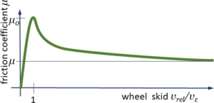
It mimics the key properties of dry friction with a stick-coefficient μ₀ for very low relative velocities and μ else. To simplify implementation, we’ll be using the same mechanism as for the tracks to compose this characteristic from lines and transition parabolas.

The latter part for F_L represents a force that is required to push the elastic wheel through elasto-plastic ground. We'll keep it simple and phrase it to be

$F_{L}=\mu \cdot N_{a}\cdot {\frac {\displaystyle 2}{\displaystyle \pi }}{\text{atan}}\left({\frac {\displaystyle v_{T}}{\displaystyle v_{T0}}}\right)$

with the new loss-velocity v_T0. The atan-function looks somewhat displaced here - it ensures that the rolling loss-force does not exceed the traction force.

Model

For this geometrically nonlinear system, it is a challenge to derive the equations of motion. We’ll be employing the Principle of Virtual Work with the equilibrium condition stating that the sum of all virtual work at the point of equilibrium vanishes:

${\begin{array}{ll}\delta W&=\delta W^{a}-\delta \Pi \\&{\stackrel {!}{=}}0\end{array}}$

with the virtual strain energy δΠ and the virtual work of external forces δW^a. These equilibrium conditions will deliver the nonlinear equations of motion for the minimal-coordinates of the car

${\underline {q}}_{C}(t):=\left({\begin{array}{c}u_{1}(t)\\u_{2}(t)\\u_{3}(t)\\u_{4}(t)\\\varphi (t)\\\psi (t)\end{array}}\right)$.

The inertia-forces for the equilibrium conditions result form accelerations, i.e. second order time-derivatives of these coordinates. Thus, we have their velocities as further state variables. Well, except for the wheel-rotation-angle ψ(t), which we are not interested in. With

${\frac {\displaystyle \psi (t)}{\displaystyle dt}}=:\omega (t)$

we collect all state variables of the system as

${\underline {Q}}_{C}(t):=\left({\begin{array}{c}{\frac {\displaystyle du_{1}(t)}{\displaystyle dt}}\\{\frac {\displaystyle du_{2}(t)}{\displaystyle dt}}\\{\frac {\displaystyle du_{3}(t)}{\displaystyle dt}}\\{\frac {\displaystyle du_{4}(t)}{\displaystyle dt}}\\{\frac {\displaystyle d\varphi (t)}{\displaystyle dt}}\\\omega (t)\\u_{1}(t)\\u_{2}(t)\\u_{3}(t)\\u_{4}(t)\\\varphi (t)\end{array}}\right)$.

When deriving the equations of motion with the principle of virtual displacements we also need the variations of r_C, r_A, r_B with respect to Q_C,. They come from

$\delta {\underline {r}}_{J}(q_{C,1},\ldots ,q_{C,i},\ldots ,q_{C,6})=\displaystyle \sum _{j=1}^{6}\left.{\frac {\displaystyle \partial {\underline {r}}_{J}(q_{C,1},\ldots ,q_{C,j}+\varepsilon \cdot \delta q_{C,j},\ldots ,q_{C,6})}{\displaystyle \partial \varepsilon }}\right\vert _{\;\displaystyle \varepsilon =0},J\in \left\{A,B,C\right\}$,

thus

$\delta {\underline {r}}_{M}=\left({\begin{array}{c}\delta u_{1}\\\delta u_{2}\end{array}}\right)$,

$\delta {\underline {r}}_{A}={\begin{pmatrix}-{a_{1}}\sin {\left(\operatorname {\varphi } (t)\right)}{\mathit {\delta \varphi }}-\left({u_{3}}(t)-{a_{3}}\right)\cos {\left(\operatorname {\varphi } (t)\right)}{\mathit {\delta \varphi }}-{{\mathit {\delta u}}_{3}}\sin {\left(\operatorname {\varphi } (t)\right)}+{{\mathit {\delta u}}_{1}}\\-\left({u_{3}}(t)-{a_{3}}\right)\sin {\left(\operatorname {\varphi } (t)\right)}{\mathit {\delta \varphi }}+{a_{1}}\cos {\left(\operatorname {\varphi } (t)\right)}{\mathit {\delta \varphi }}+{{\mathit {\delta u}}_{3}}\cos {\left(\operatorname {\varphi } (t)\right)}+{{\mathit {\delta u}}_{2}}\end{pmatrix}}$,

$\delta {\underline {r}}_{B}={\begin{pmatrix}{a_{2}}\sin {\left(\operatorname {\varphi } (t)\right)}{\mathit {\delta \phi }}-\left({u_{4}}(t)-{a_{3}}\right)\cos {\left(\operatorname {\varphi } (t)\right)}{\mathit {\delta \varphi }}-{{\mathit {\delta u}}_{4}}\sin {\left(\operatorname {\varphi } (t)\right)}+{{\mathit {\delta u}}_{1}}\\-\left({u_{4}}(t)-{a_{3}}\right)\sin {\left(\operatorname {\varphi } (t)\right)}{\mathit {\delta \varphi }}-{a_{2}}\cos {\left(\operatorname {\varphi } (t)\right)}{\mathit {\delta \varphi }}+{{\mathit {\delta u}}_{4}}\cos {\left(\operatorname {\varphi } (t)\right)}+{{\mathit {\delta u}}_{2}}\end{pmatrix}}$,

$\delta {\underline {r}}_{a}={\begin{pmatrix}-R\cos {\left({{\gamma }_{A}}(t)\right)}{\mathit {\delta \psi }}+\left(-{a_{1}}\sin {\left(\operatorname {\phi } (t)\right)}+\left({a_{3}}-{u_{3}}(t)\right)\cos {\left(\operatorname {\phi } (t)\right)}+R\cos {\left({{\gamma }_{A}}(t)\right)}\right)\,{\mathit {\delta \phi }}-{{\mathit {\delta u}}_{3}}\sin {\left(\operatorname {\phi } (t)\right)}+{{\mathit {\delta u}}_{1}}\\-R\sin {\left({{\gamma }_{A}}(t)\right)}{\mathit {\delta \psi }}+\left(\left({a_{3}}-{u_{3}}(t)\right)\sin {\left(\operatorname {\phi } (t)\right)}+{a_{1}}\cos {\left(\operatorname {\phi } (t)\right)}+R\sin {\left({{\gamma }_{A}}(t)\right)}\right)\,{\mathit {\delta \phi }}+{{\mathit {\delta u}}_{3}}\cos {\left(\operatorname {\phi } (t)\right)}+{{\mathit {\delta u}}_{2}}\end{pmatrix}}$

and - not accounting for ψ and κ - as

$\delta {\underline {r}}_{b}={\begin{pmatrix}{a_{2}}\sin {\left(\operatorname {\varphi } (t)\right)}{\mathit {\delta \varphi }}-\left({u_{4}}(t)-{a_{3}}\right)\cos {\left(\operatorname {\varphi } (t)\right)}{\mathit {\delta \varphi }}-{{\mathit {\delta u}}_{4}}\sin {\left(\operatorname {\varphi } (t)\right)}+{{\mathit {\delta u}}_{1}}\\-\left({u_{4}}(t)-{a_{3}}\right)\sin {\left(\operatorname {\varphi } (t)\right)}{\mathit {\delta \varphi }}-{a_{2}}\cos {\left(\operatorname {\varphi } (t)\right)}{\mathit {\delta \varphi }}+{{\mathit {\delta u}}_{4}}\cos {\left(\operatorname {\varphi } (t)\right)}+{{\mathit {\delta u}}_{2}}\end{pmatrix}}$.

Virtual Strain Energy

The only elastic elements in our car are the two springs, thus

$\delta \Pi =k_{A}\cdot u_{3}\cdot \delta u_{3}+k_{B}\cdot u_{4}\cdot \delta u_{4}$.

/* in next section ... */

Virtual Work of External Forces - including D'Alembert Forces

The components of virtual work of external forces are

$\delta W^{a}=\delta W_{g}^{a}+\delta W_{A}^{a}+\delta W_{d}^{a}+\delta W_{F}^{a}$

where

• δW^a_g: virtual work of gravitational forces,
• δW^a_A: virtual work of D'Alembert inertia forces,
• δW^a_d: virtual work of dissipative forces (dampers parallel to the suspension springs / rotational damping) and
• 'δW^a_F': virtual work of implied forces and moments like N_A, N_B, F and M_W.

With the principle of virtual work, we phrase

$\delta W_{g}^{a}=-m_{C}\;g\;{\vec {e}}_{y}\cdot \delta {\vec {r}}_{C}-m_{A}\;g\;{\vec {e}}_{y}\cdot \delta {\vec {r}}_{A}-m_{B}\;g\;{\vec {e}}_{y}\cdot \delta {\vec {r}}_{B}$,

$\delta W_{A}^{a}=-m_{C}\;{\ddot {\vec {r}}}_{C}\cdot \delta {\vec {r}}_{C}-m_{A}\;{\ddot {\vec {r}}}_{A}\cdot \delta {\vec {r}}_{A}-m_{B}\;{\ddot {\vec {r}}}_{B}\cdot \delta {\vec {r}}_{B}-J_{C}\;{\ddot {\varphi }}\cdot \delta \varphi -J_{A}\;{\ddot {\psi }}\cdot \delta \psi$,

$\delta W_{d}^{a}=b_{3}\,{\dot {u}}_{3}\cdot \delta u_{3}+b_{4}\,{\dot {u}}_{4}\cdot \delta u_{4}+B\,\left(\omega (t)+\Omega (t)\right)\cdot \left(\delta \psi +\delta \varphi \right)$

and

$\delta W_{F}^{a}={\underline {\underline {D}}}(\gamma _{A})\cdot \left({\begin{array}{c}T\\N_{A}\end{array}}\right)\cdot \delta {\underline {r}}_{a}+{\underline {\underline {D}}}(\gamma _{B})\cdot \left({\begin{array}{c}0\\N_{B}\end{array}}\right)\cdot \delta {\underline {r}}_{b}+M_{W}\cdot \delta \psi ;$.

We group all components of by their virtual displacements , the coefficient of each virtual displacement being one equilibrium condition. The resultant equations have this form:

$\delta W=\delta {\underline {q}}_{C}\cdot \left(-{\underline {\underline {M}}}\cdot {\ddot {\underline {q}}}+{\underline {f}}({\dot {\underline {q}}},{\underline {q}})\right)$.

/*******************************************************/
/* MAXIMA script                                       */
/* version: wxMaxima 16.04.2                           */
/* author: Andreas Baumgart                            */
/* last updated: 2021-02-08                            */
/* ref: Modelling and Simulation (TUAS)                */
/* description: Rounding between straight line-segments*/
/*******************************************************/

/*******************************************************/
/* declarations                                        */
/*******************************************************/
declare("λ", alphabetic);
declare("Δ", alphabetic);
declare("δ", alphabetic,"ε", alphabetic);
declare("Π", alphabetic);
declare("φ", alphabetic);
declare("ψ", alphabetic);
declare("κ", alphabetic);
declare("α", alphabetic);
declare("γ", alphabetic);
declare("ω", alphabetic);

/*******************************************************/
/* body centers                                        */
/*******************************************************/
/* car body */
r[C] : [u[1](t),u[2](t)];
D[1](α) := matrix([cos(α),-sin(α)],[sin(α),cos(α)]);

/* wheel centers - reference configuration */
r[A] : r[C] + D[1](φ(t)).matrix([+a[1]],[-a[3]+u[3](t)]);
r[B] : r[C] + D[1](φ(t)).matrix([-a[2]],[-a[3]+u[4](t)]);

/* wheel contacts */

local : [γ[A](t) = φ(t) + (κ(t)-ψ(t))];
r[a] : r[A] + D[1](γ[A](t)).matrix([0],[-R]);
r[b] : r[B] + D[1](γ[B](t)).matrix([0],[-R]);

varia: append(makelist(u[i](t) =  u[i](t) + ε*δu[i],i,1,4),[φ(t) = φ(t) + ε*δφ, ψ(t) = ψ(t) + ε*δψ]); 

q  : append(makelist( u[i](t),i,1,4), [ φ(t), ψ(t)]);
δq : append(makelist(δu[i]   ,i,1,4), [δφ   ,δψ   ]);
nuller : makelist(q[i]=0, i,1,length(q));

δr[C] : sum(subst([ε=0],diff(subst(varia[i],r[C]),ε)),i,1,length(varia));
δr[A] : sum(subst([ε=0],diff(subst(varia[i],r[A]),ε)),i,1,length(varia));
δr[B] : sum(subst([ε=0],diff(subst(varia[i],r[B]),ε)),i,1,length(varia));
δr[a] : sum(subst([ε=0],diff(subst(varia[i],subst(local,r[a])),ε)),i,1,length(varia));
δr[b] : sum(subst([ε=0],diff(subst(varia[i],subst(local,r[b])),ε)),i,1,length(varia));

/* d'Alembert Forces */
δW[I] : expand(-m[1]*diff(r[C],t,2).δr[C] - m[2]*diff(r[A],t,2).δr[A] - m[2]*diff(r[B],t,2).δr[B] - J[1]*diff(φ(t),t,2)*δφ - J[2]*diff(ψ(t),t,2)*δψ);
δW[I] : expand(subst(['diff(φ(t),t,1)^2=0],δW[I]));

/* Springs / Dampers*/
δΠ : (k[1]*u[3](t)+b[1]*diff(u[3](t),t))*δu[3]+(k[2]*u[4](t)+b[2]*diff(u[4](t),t))*δu[4];
δΠ : expand(δΠ);

/* Motor (δφ has the opposite orientation of δψ) */
δW[m] : MW*δψ;

/* Weight */
δW[G] : -m[1]*g*δu[2] - m[2]*g*δr[A][2] - m[2]*g*δr[B][2];

/* Contact*/
δW[c] : δr[a].(D[1](γ[A]).[F[T],F[N1]]) + δr[b].(D[1](γ[2]).[0,F[N2]]);
δW[c] : expand(subst(solve(local,κ(t))[1],δW[c]));

/*--------------------------------------------------*/
δW[total] : expand(δW[I] - δΠ + δW[G] + δW[c] + δW[m]);

eom : expand(makelist(coeff(δW[total][1],δq[i]),i,1,length(δq)));
δW[rest] : expand(δW[total][1] -sum(eom[i]*δq[i],i,1,length(δq)));

M : funmake('matrix,makelist(makelist(coeff(eom[row],diff(q[col],t,2)),col,1,length(q)),row,1, length(q)));
trigRepl : [solve(cos(γ[B]-φ(t)) = trigexpand(cos(γ[B]-φ(t))),sin(γ[B]))[1],
            solve(cos(γ[A]-φ(t)) = trigexpand(cos(γ[A]-φ(t))),sin(γ[A]))[1],
            solve(sin(γ[A]-φ(t)) = trigexpand(sin(γ[A]-φ(t))),cos(γ[A]))[1]];

rightHandS : expand(makelist(eom[row] - sum(M[row,col]*diff(q[col],t,2),col,1,length(q)),row,1, length(q)));
/* neglect the impact of deflections u[3], u[4] on the mass moment of the total car */
/* further simplifications of intertial forces */
rightHandS[1]:ratsimp(trigsimp(subst(['diff(u[3](t),t,1)=0,'diff(u[4](t),t,1)=0],rightHandS[1])));
rightHandS[2]:ratsimp(trigsimp(subst(['diff(u[3](t),t,1)=0,'diff(u[4](t),t,1)=0],rightHandS[2])));

tmp          : F[N1]*subst(trigRepl[2],coeff(rightHandS[3],F[N1]))+
               F[T] *subst(trigRepl[3],coeff(rightHandS[3],F[T] ));
rightHandS[3]: tmp+ratsimp(trigexpand(rightHandS[3]-tmp));
rightHandS[4]: ratsimp(subst(trigRepl,rightHandS[4]));

rightHandS[5]:subst(['diff(u[3](t),t,1)=0,'diff(u[4](t),t,1)=0],rightHandS[5]);
trigRepl : [cos(γ[A]-φ(t)) = trigexpand(cos(γ[A]-φ(t))),
            cos(γ[B]-φ(t)) = trigexpand(cos(γ[B]-φ(t))),
	    sin(γ[A]-φ(t)) = trigexpand(sin(γ[A]-φ(t))),
	    sin(γ[B]-φ(t)) = trigexpand(sin(γ[B]-φ(t)))];
/* need to get rid of the Minus-signs .... */
assume(cos(γ[A])>0,cos(γ[B])>0,sin(γ[A])>0,sin(γ[B])>0,sin(φ(t))>0,cos(φ(t))>0);
for i:1 thru 4 do
    (trigRepl[i] : trigRepl[i] - part(rhs(trigRepl[i]),1),
     trigRepl[i] : rhs(trigRepl[i]) = lhs(trigRepl[i]),
     if is(lhs(trigRepl[i])<0) then
     	trigRepl[i] : -trigRepl[i]);
abbrev : solve([a[3]-u[3](t)=Δu[3], a[3]-u[4](t)=Δu[3]],[u[3](t),u[4](t)])[1];
collector : [[F[N1],F[N2],F[T]],[a[1],a[2],a[3]]];
tmp : makelist(makelist(coeff(coeff(rightHandS[5],collector[1][i]),collector[2][j]),j,1,3),i,1,3);
tmp : subst(trigRepl,tmp);
tmp : sum(sum(tmp[i][j]*collector[1][i]*collector[2][j],j,1,3),i,1,3);
rightHandS[5]: trigsimp(ratsimp(expand(tmp+ratsimp(trigexpand(rightHandS[5]-tmp)))));

/* ... now simplify mass matrix */
M : -subst(nuller,M);
for row:1 thru 5 do
    (for col:row thru 5 do
    	print("M(",row,",",col,") = ",M[row][col]))$

/* and print right-hand-side */
for i:1 thru length(q)  do
   (grind(trigsimp(ratsimp(rightHandS[i]))),
    print("---------------------------------------------------"))$

/* tnslate */
toDyDt : [cos(γ[A]) = cosgamma[1],cos(γ[B]) = cosgamma[2],
          sin(γ[A]) = singamma[1],sin(γ[B]) = singamma[2],
	  cos(φ(t)) = cosphi, sin(φ(t)) = sinphi, 	  
          'diff(u[3](t),t,1) = v[3],	  
          'diff(u[4](t),t,1) = v[4]]
for i:1 thru length(q)  do
   (print(trigsimp(ratsimp(subst(toDyDt,rightHandS[i])))),
    print("---------------------------------------------------"))$
/************************************************************************/
/* start vector */
starter : append(makelist('diff(u[i](t),t,1)=0,i,1,4),
   	       	 [sin(φ(t))=0,cos(φ(t))=1,'diff(φ(t),t,1)=0],
	       	 [F[N1]=0,F[N2]=0,F[T]=0, MW=0]);

atStart : makelist(subst(starter,eom)[i]=0,i,1,length(q));
TT : append(makelist(diff(u[i](t),t,2),i,1,4),['diff(φ(t),t,2),'diff(ψ(t),t,2)]);
START : solve(atStart, TT)[1];

makelist(lhs(START[i])=subst([u[3](t)=0,u[4](t)=0],rhs(START[i])),i,1,length(q));

/************************************************************************/
/* translate to first-order DGL */
toDyDt: ['diff(u[1](t),t,1) = Q[ 1],
      	 'diff(u[2](t),t,1) = Q[ 2],
      	 'diff(u[3](t),t,1) = Q[ 3],
      	 'diff(u[4](t),t,1) = Q[ 4],
      	 'diff(   φ(t),t,1) = Q[ 5],
      	 'diff(   ψ(t),t,1) = Q[ 6],
	       u[1](t) 	    = Q[ 7],
      	       u[2](t) 	    = Q[ 8],
      	       u[3](t) 	    = Q[ 9],
      	       u[4](t) 	    = Q[10],
      	       φ(t)    	    = Q[11],
      	    sin(Q[11])      = sinphi,
      	    cos(Q[11])      = cosphi];

rhside : ratsimp(subst(toDyDt,rightHandS));

for i:1 thru 6  do
   (print("rhs(",i,") = ",ratsimp(rhside[i])),
    print("---------------------------------------------------"))$


taylor : [cos(φ(t)) = 1-φ(t)^2/2!,sin(φ(t)) = φ(t)-φ(t)^3/3!];plot2d([sin(phi), phi-phi^3/3!],[phi, -%pi/2, %pi/2])$



/* velocity in contact point */
/* of axles ..... */
/* im Reference-System */
v[A] : trigsimp(diff(r[A],t));
v[B] : trigsimp(diff(r[B],t));

/* Transformation ins surface-system*/
V[a] : D[1](-γ[A]).[V[3],V[4]]+[-R*ω,0];
V[v] : D[1](-γ[B]).[V[5],V[6]];

/***************************** using formal approach ******************************/
/* in reference-coordinates */
/* axle "1" */
reverse : solve(local,κ(t))[1];
v[a] : subst([reverse, diff(reverse,t)], diff(subst(local,r[a]),t));
v[a] : subst([diff(ψ(t),t)=ω(t)], subst(subst(['diff(κ(t),t,1)=0],diff(local,t,1)), ev(v[a],nouns)));
/* in surface - coordinates */
V[a] : trigsimp(expand(D[1](-γ[A]).v[a]));

/* axle "2" */
v[b] : diff(subst(local,r[b]),t);
/* in surface - coordinates */
V[b] : trigsimp(expand(D[1](-γ[B]).v[b]));

The components of this equation are

${\underline {\underline {M}}}={\begin{pmatrix}2{m_{2}}+{m_{1}}&0&0&0&2{m_{2}}\,{a_{3}}&0\\0&2{m_{2}}+{m_{1}}&{m_{2}}&{m_{2}}&{a_{1}}\,{m_{2}}-{a_{2}}\,{m_{2}}&0\\0&{m_{2}}&{m_{2}}&0&{a_{1}}\,{m_{2}}&0\\0&{m_{2}}&0&{m_{2}}&-{a_{2}}\,{m_{2}}&0\\2{m_{2}}\,{a_{3}}&{a_{1}}\,{m_{2}}-{a_{2}}\,{m_{2}}&{a_{1}}\,{m_{2}}&-{a_{2}}\,{m_{2}}&2{m_{2}}\,{{a}_{3}^{2}}+{{a}_{2}^{2}}\,{m_{2}}+{{a}_{1}^{2}}\,{m_{2}}+{J_{1}}&0\\0&0&0&0&0&{J_{2}}\end{pmatrix}}$

and

${\underline {f}}=\left({\begin{array}{l}\cos {\left({{\gamma }_{A}}\right)}{F_{T}}-\sin {\left({{\gamma }_{2}}\right)}{F_{\mathit {N2}}}-\sin {\left({{\gamma }_{A}}\right)}{F_{\mathit {N1}}}\\\left(-2{m_{2}}-{m_{1}}\right)g+\sin {\left({{\gamma }_{A}}\right)}{F_{T}}+\cos {\left({{\gamma }_{2}}\right)}{F_{\mathit {N2}}}+\cos {\left({{\gamma }_{A}}\right)}{F_{\mathit {N1}}}\\-{F_{T}}\sin {\left(\operatorname {\varphi } (t)-{{\gamma }_{A}}\right)}+{F_{\mathit {N1}}}\cos {\left(\operatorname {\varphi } (t)-{{\gamma }_{A}}\right)}-{m_{2}}g\cos {\left(\operatorname {\varphi } (t)\right)}-{b_{1}}\,{\dot {u}}_{3}-{k_{1}}{u_{3}}(t)\\\sin {\left({{\gamma }_{2}}\right)}{F_{\mathit {N2}}}\sin {\left(\operatorname {\varphi } (t)\right)}+\left(\cos {\left({{\gamma }_{2}}\right)}{F_{\mathit {N2}}}-{m_{2}}g\right)\cos {\left(\operatorname {\varphi } (t)\right)}-{b_{2}}\,{\dot {u}}_{4}-{k_{2}}{u_{4}}(t)\\\left({a_{3}}\,{F_{\mathit {N1}}}-{a_{1}}\,{F_{T}}\right)\sin {\left(\operatorname {\varphi } (t)-{{\gamma }_{A}}\right)}+\left({a_{3}}\,{F_{T}}+{a_{1}}\,{F_{\mathit {N1}}}\right)\cos {\left(\operatorname {\varphi } (t)-{{\gamma }_{A}}\right)}+\sin {\left(\operatorname {\varphi } (t)\right)}+\left(\sin {\left({{\gamma }_{2}}\right)}{F_{\mathit {N2}}}{u_{4}}(t)+\left(\sin {\left({{\gamma }_{A}}\right)}{F_{\mathit {N1}}}-\cos {\left({{\gamma }_{A}}\right)}{F_{T}}\right){u_{3}}(t)+\left({a_{2}}-{a_{1}}\right)\,{m_{2}}g+\left(-{a_{3}}\sin {\left({{\gamma }_{2}}\right)}-{a_{2}}\cos {\left({{\gamma }_{2}}\right)}\right)\,{F_{\mathit {N2}}}\right)\cos {\left(\operatorname {\varphi } (t)\right)}+\left(\sin {\left({{\gamma }_{A}}\right)}R\,{F_{T}}+\cos {\left({{\gamma }_{A}}\right)}{F_{\mathit {N1}}}R\right)\sin {\left({{\gamma }_{A}}(t)\right)}+\left(\cos {\left({{\gamma }_{A}}\right)}R\,{F_{T}}-\sin {\left({{\gamma }_{A}}\right)}{F_{\mathit {N1}}}R\right)\cos {\left({{\gamma }_{A}}(t)\right)}+B\,\left(\omega (t)+\Omega (t)\right)\\\left(-\sin {\left({{\gamma }_{A}}\right)}R\,{F_{T}}-\cos {\left({{\gamma }_{A}}\right)}{F_{\mathit {N1}}}R\right)\sin {\left({{\gamma }_{A}}(t)\right)}+\left(\sin {\left({{\gamma }_{A}}\right)}{F_{\mathit {N1}}}R-\cos {\left({{\gamma }_{A}}\right)}R\,{F_{T}}\right)\cos {\left({{\gamma }_{A}}(t)\right)}+B\,\left(\omega (t)+\Omega (t)\right)+M_{W}\end{array}}\right)$

Later we’ll see that this representation has a small structural fault: the wheel torque M_W depends on the angular acceleration of the motor and gears. It implies that M_W is a function of

${\ddot {\psi }}(t){\text{ or }}{\dot {\omega }}(t)$

and needs to be transferred to the left-hand-side of the equations. That fault will be corrected when the E-Motor and Drive-Train-components are integrated.

Variables

name	symbol	unit
u1	center of mass displacement in x-direction	m
u2	center of mass displacement in y-direction	m
u3	spring compression at front axis	m
u4	spring compression at rear axis	m
ϕ	rotation of car-body	rad
ψ	rotation of wheel (absolute - not relative to car-body)	rad

Parameter

name	symbol	value	unit
axis distance	a0	40	cm
distance front axis center of mass	a1	10	cm
vertical distance from wheel-hub to center of mass for relaxed springs	a3	10	cm
wheel radius	R	58.42	mm
car-body mass	mC	4	kg
wheel-set mass	mW	0.3	kg
inertia-radius for body with $J_{C}=m_{C}\cdot r_{C}^{2}$	rC	15	cm
inertia-radius wheel-set	rW	4	cm
track-stiffness	kT	1.00E+04	N/m
spring stiffness front	k1	500	N/m
spring stiffness rear; if "0" is given, compute it so that the static ϕ=0	k2	0	N/m
spring damping front	b1	100	N/(m/s)
spring damping rear	b2	100	N/(m/s)
smoothening radius for spring characteristic	ε	1	mm
friction coefficient	μ	0.4	1
rounding radius for friction coefficient	με	0.01	1
stick coefficient	μ0	0.6	1
reference velocity for damping at springs	vref	5	m/s
loss velocity for rolling contact	vT0	5	m/s

next workpackage: driver-controls →

---

References

• ...