Gelöste Aufgaben/JUMP/Battery: Unterschied zwischen den Versionen
| (5 dazwischenliegende Versionen desselben Benutzers werden nicht angezeigt) | |||
| Zeile 78: | Zeile 78: | ||
::<math>\begin{array}{lcl} | ::<math>\begin{array}{lcl} | ||
e(S_D) &:= &\frac{\displaystyle E(Q_B)}{\displaystyle U_0}\\ | e(S_D) &:= &\frac{\displaystyle E(Q_B)}{\displaystyle U_0}\\ | ||
&=&\displaystyle \sum_0^ | &=&\displaystyle \sum_0^5 C_i \cdot S_D^i | ||
\end{array}</math> | \end{array}</math> | ||
| Zeile 205: | Zeile 205: | ||
::<math>\begin{array}{ll} | ::<math>\begin{array}{ll} | ||
\dot{Q}_H &= R_1\cdot I_B^2 + R_{ | \dot{Q}_H &= R_1\cdot I_B^2 + R_{2} \cdot I_2^2 \text{ where } I_{2} = \frac{\displaystyle U_2}{\displaystyle R_2}\\ | ||
U_B &= R_1 \cdot I_B + U_{2} + E(S_D),\\ | U_B &= R_1 \cdot I_B + U_{2} + E(S_D),\\ | ||
\dot{Q}_D &= H_B \cdot (T_B(t) - T_0). | \dot{Q}_D &= H_B \cdot (T_B(t) - T_0). | ||
| Zeile 232: | Zeile 232: | ||
The coefficients ''C<sub>i</sub>'' for ''e(S<sub>D</sub>)'' have been computed from conditions for a 5th-order polynomial by defining function-values and gradients at reference points: | The coefficients ''C<sub>i</sub>'' for ''e(S<sub>D</sub>)'' have been computed from conditions for a 5th-order polynomial by defining function-values and gradients at reference points: | ||
<math>C_0=\frac{11}{10},C_1=-1,C_2=\frac{1177}{240},C_3=-\frac{28489}{2160},C_4=\frac{7891}{432},C_5=-\frac{4355}{432}</math>[[Datei:JUMP-battery-characteristic-implemented.png|mini|Implemented Characteristic]]The plot right shows the resultant characteristic of ''e(S<sub>D</sub>)'': | ::<math>C_0=\frac{11}{10},C_1=-1,C_2=\frac{1177}{240},C_3=-\frac{28489}{2160},C_4=\frac{7891}{432},C_5=-\frac{4355}{432}</math> | ||
[[Datei:JUMP-battery-characteristic-implemented.png|mini|Implemented Characteristic]] | |||
The plot right shows the resultant characteristic of ''e(S<sub>D</sub>)'': | |||
For the remaining parameters, no measurements were available. We adopted those to obtain a performance similar to what has been described in [1], the resistors were chosen as to “deliver” reasonable amounts of heat when the battery is discharged with rating of C=25. | For the remaining parameters, no measurements were available. We adopted those to obtain a performance similar to what has been described in [1], the resistors were chosen as to “deliver” reasonable amounts of heat when the battery is discharged with rating of C=25. | ||
| Zeile 244: | Zeile 247: | ||
For ''α'' and ''β'' we know that their gradients | For ''α'' and ''β'' we know that their gradients | ||
<math>\frac{\displaystyle d \; \alpha}{ \displaystyle d \; I_B} > 0</math> | ::<math>\frac{\displaystyle d \; \alpha}{ \displaystyle d \; I_B} > 0</math> | ||
and | and | ||
<math>\frac{\displaystyle d\; \beta}{\displaystyle \; dT} < 0</math>. | ::<math>\frac{\displaystyle d\; \beta}{\displaystyle \; dT} < 0</math>. | ||
The reference curve from above shall be assumed to be valid for ''I<sub>B</sub>'' = 20 A and we assume | The reference curve from above shall be assumed to be valid for ''I<sub>B</sub>'' = 20 A and we assume | ||
<math>\begin{array}{lll} | ::<math>\begin{array}{lll} | ||
\alpha(I_B) &= 1 + \frac{\displaystyle I_B}{\displaystyle I_ \alpha} &\text{ with } I_\alpha = 100 A\\ | \alpha(I_B) &= 1 + \frac{\displaystyle I_B}{\displaystyle I_ \alpha} &\text{ with } I_\alpha = 100 A\\ | ||
\beta(T) &= 1 - \frac{\displaystyle T_B}{\displaystyle T_ \beta} &\text{ with } T_ \beta = 100^\circ C | \beta(T) &= 1 - \frac{\displaystyle T_B}{\displaystyle T_ \beta} &\text{ with } T_ \beta = 100^\circ C | ||
| Zeile 264: | Zeile 267: | ||
And finally ''h<sub>B</sub>'' will be identified from a (virtual) experiment: let ''I<sub>B</sub>'' = 0, ''I<sub>2</sub>''=0 (no heat generation) and the initial battery-temperature to be ''ΔT(0)'' above ''T<sub>0</sub>''. Then assume that ''ΔT(''3min'')'' is reduced to 50% of ''ΔT(0)''. From above, we find the differential equation to be | And finally ''h<sub>B</sub>'' will be identified from a (virtual) experiment: let ''I<sub>B</sub>'' = 0, ''I<sub>2</sub>''=0 (no heat generation) and the initial battery-temperature to be ''ΔT(0)'' above ''T<sub>0</sub>''. Then assume that ''ΔT(''3min'')'' is reduced to 50% of ''ΔT(0)''. From above, we find the differential equation to be | ||
<math>\Delta T(t)= \Delta T_0 \cdot \text{e}^{-\frac{\displaystyle h_B \cdot t}{\displaystyle m_B \cdot c_{PB}}}</math>, | ::<math>\Delta T(t)= \Delta T_0 \cdot \text{e}^{-\frac{\displaystyle h_B \cdot t}{\displaystyle m_B \cdot c_{PB}}}</math>, | ||
thus for this “experiment” | thus for this “experiment” | ||
<math>h_B=(\text{log}(2) \cdot m_B\cdot c_{PB})/ 3 \text{ min}</math>. | ::<math>h_B=(\text{log}(2) \cdot m_B\cdot c_{PB})/ 3 \text{ min}</math>. | ||
With the values given above, we find | With the values given above, we find | ||
''h<sub>B</sub>=2.6E-3 J/(K''s) | ::''h<sub>B</sub>=2.6E-3 J/(K''s) | ||
Let the tolerable, maximum battery temperature be | Let the tolerable, maximum battery temperature be | ||
<math>T_{B,max} = 60^\circ C</math>. | ::<math>T_{B,max} = 60^\circ C</math>. | ||
{| class="wikitable" style="border-collapse: collapse;" | |||
!style="border-right: solid 0px;"|name | |||
!symbol | |||
!value | |||
!unit | |||
|- | |||
|battery mass | |||
|''m<sub>B</sub>'' | |||
|340 | |||
|g | |||
|- | |||
|specific heat capacity (averaged) | |||
|''c<sub>pB</sub>'' | |||
|1015 | |||
|J/(kg*K) | |||
|- | |||
|resistor 1 | |||
|''R<sub>1</sub>'' | |||
|0.05 | |||
|Ω | |||
|- | |||
|resistor 2 | |||
|''R<sub>2</sub>'' | |||
|0.025 | |||
|Ω | |||
|- | |||
|capacity | |||
|''Q<sub>B0</sub>'' | |||
|5000 | |||
|Ah | |||
|- | |||
|battery discharge rating | |||
|''1C'' | |||
|25 | |||
|A | |||
|- | |||
|battery reference potential voltage | |||
|''U<sub>0</sub>'' | |||
|8 | |||
|V | |||
|- | |||
|ambient temperature | |||
|''T<sub>0</sub>'' | |||
|20 | |||
|°C | |||
|- | |||
|time it takes to let the battery cool down by 50% | |||
|''T<sub>50</sub>'' | |||
|180 | |||
|s | |||
|- | |||
|correction value for current ''I<sub>B</sub>'' | |||
|''I<sub>α</sub>'' | |||
|100 | |||
|A | |||
|- T[beta] 100 | |||
|correction value for current ''T<sub>B</sub>'' | |||
|''T<sub>β</sub>'' | |||
|100 | |||
|°C | |||
|} | |||
<hr/> | |||
[[Gelöste Aufgaben/JUMP/Car-Body|next workpackage: car-body →]] | [[Gelöste Aufgaben/JUMP/Car-Body|next workpackage: car-body →]] | ||
Aktuelle Version vom 22. März 2021, 07:57 Uhr
Scope

The battery is our power-supply. Depending on the discharging current IB consumed by our drive-train, the battery will display a voltage UB.
We are looking for a mathematical model that accounts for discharging operations only and we are not interested in high-frequency load-idle-cycles. Long-term changes of battery-parameters are out of scope.
We copy the typical specifications for a LiPo battery used for RC Model Cars to be:
- total capacity: QB0 = 5000 mAh,
- voltage: UB0 = 11.1 V,
- C-rating: 25.
The C-rating refers to the rate of energy the battery can safely discharge continuously, represented in terms of current as a multiple of its overall capacity. The maximum continuous current for this battery is
Also we need to model the battery heat to avoid excessive temperatures TB of the battery.
Structure
Our model accounts for two aspects:
- power delivery and
- temperature.
Both aspects are related in the sense that discharging operations with high currents lead to high battery-temperatures which will reduce the effective battery capacity.
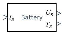
The equivalent block-diagram of our model is this:
The battery-current IB entails a battery voltage UB and Temperature TB.
Power Delivery

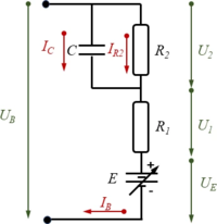
We employ a standard battery model which accounts for
- E: the equilibrium potential
- R1, R2: two internal resistances and
- C: an effective capacitance.
In a steady-state-condition, the battery voltage UB is thus a function of the battery current IB.
Temperature

Our simple lumped-body model accounts for heat generation inside the battery and heat dissipation over its surface.
In steady-state condition, they are equal, if heat generation exceeds heat dissipation , the battery heat increases - und thus its temperature.
Model
Power Delivery
Using Kirchhoff’s laws and from the model-diagram of the electric-circuit of the battery, we find the equilibrium conditions
- .
The potential E is a function of the effective battery capacity or the commonly used dimensionless “state of dischange”
- .

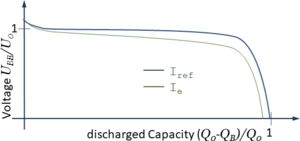
E(SD) depends in a complex way on the electrochemical processes within the battery. We account for this functional relationship using a characteristic curve which we copy from literature.
In operation, the reference battery capacity QB0 is being consumed by the current IB, thus
- ,
where α is a correction-factor accounting for the current IB and β accounting for the battery-temperature TB. The effect of α can be seen in the diagram above where Ie > Iref.
For a representation of this function, we choose an appropriate polynomial with
Its unknown coefficients Ci will be identified from the characteristic above. The components of the electric circuit provide these equations
with α, β being current- and temperature-related correction factors respectively.
With the nominal battery capacity QB0 and the actual capacity QB, we have the commonly employed state of discharge SD to be
/*******************************************************/
/* MAXIMA script                                       */
/* version: wxMaxima 18.10.1                           */
/* author: Andreas Baumgart                            */
/* last updated: 2021-02-08                            */
/* ref: Modelling and Simulation (TUAS)                */
/* description: Rounding between straight line-segments*/
/*******************************************************/

/*******************************************************/
/* declarations                                        */
/*******************************************************/
declare("ω",alphabetic);
declare("α",alphabetic);
declare("β",alphabetic);

/*******************************************************/
/* equations of motion                                 */
/*******************************************************/
/* Kirchhoff's law     */
KL : [U[0] = E+U[1]+U[2],
      U[1] = R[1]*I[1],
      U[2] = R[2]*I[2],
      I[1] = I[2]+I[C],
      I[C] = C*'diff(U[2],t),
      'diff(Q[B],t) = α*β*I[1],
      s = Q[B]/Q[R],
      /*             */
      m[B]*c[PB]*'diff(T[B],t)=R[1]*I[1]^2+R[2]*I[2]^2-H[B]*(T[B]-T[0])];

battery: ratsimp([subst(KL[2],KL[1]),
                  subst(solve(KL[3],I[2]), subst(solve(KL[4],I[C]), solve(KL[5],'diff(U[2],t))[1])),
		  KL[6],KL[7],KL[8]]);

/* Characteristic curve for E */
/*                            */
E(s) := sum(c[i]*s^i,i,0,5);

bc : [subst([s=0],E(s))=V[0],E(1)=0,
      subst([s=0],diff(E(s),s))=S[0],subst([s=1],diff(E(s),s))=S[2],
      E(6/10)=V[1],subst([s=6/10],diff(E(s),s))=S[1]];

params: [V[0]=4,S[0]=-1.5,V[1]=3.7,S[1]=-0.4,S[2]=-30];

sol : solve(subst(params,bc),makelist(c[i],i,0,5))[1];
plot2d(subst(sol,E(s)),[s,0,1], [xlabel,"SoD"], [ylabel,"U[0]"]);
Temperature
The thermodynamic balance-equation of heat yields
- .
| ✔ Nomenclature "Q": |
| Note that Q is used here as the heat of the battery – not as the battery-capacity as above! |
The battery heat is a function of
- temperature TB,
- averaged specific heat capacity cp,B and
- battery mass mB.
so that
- .
Heat generation inside the battery be
- .
and heat dissipation
with ambient air temperature T0 and the coefficient of heat transfer hB.
/* none given */
Summary
Thus, the battery-coordinates are
with the associated equations of motion
and additional algebraic equation
Variables
| name | symbol | unit |
|---|---|---|
| battery remaining capacity | QB | A h |
| capacitance voltage | UB2 | V |
| battery temperature | TB | °C |
Parameters
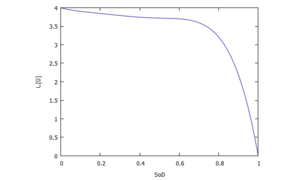
The coefficients Ci for e(SD) have been computed from conditions for a 5th-order polynomial by defining function-values and gradients at reference points:

The plot right shows the resultant characteristic of e(SD):
For the remaining parameters, no measurements were available. We adopted those to obtain a performance similar to what has been described in [1], the resistors were chosen as to “deliver” reasonable amounts of heat when the battery is discharged with rating of C=25.
- R1 = 500 mΩ
- R2 = 250 mΩ
- C = 500 F
- QB0 = 5000 Ah
- T0 = 20°C
For α and β we know that their gradients
and
- .
The reference curve from above shall be assumed to be valid for IB = 20 A and we assume
Then, for the thermal model we have
- mB = 340 g,
- cp,B = 2 J/(kg K).
And finally hB will be identified from a (virtual) experiment: let IB = 0, I2=0 (no heat generation) and the initial battery-temperature to be ΔT(0) above T0. Then assume that ΔT(3min) is reduced to 50% of ΔT(0). From above, we find the differential equation to be
- ,
thus for this “experiment”
- .
With the values given above, we find
- hB=2.6E-3 J/(Ks)
Let the tolerable, maximum battery temperature be
- .
| name | symbol | value | unit |
|---|---|---|---|
| battery mass | mB | 340 | g |
| specific heat capacity (averaged) | cpB | 1015 | J/(kg*K) |
| resistor 1 | R1 | 0.05 | Ω |
| resistor 2 | R2 | 0.025 | Ω |
| capacity | QB0 | 5000 | Ah |
| battery discharge rating | 1C | 25 | A |
| battery reference potential voltage | U0 | 8 | V |
| ambient temperature | T0 | 20 | °C |
| time it takes to let the battery cool down by 50% | T50 | 180 | s |
| correction value for current IB | Iα | 100 | A |
| correction value for current TB | Tβ | 100 | °C |
References
- Lijun Gao, Shengyi Liu; Roger A. Dougal: Dynamic Lithium-Ion Battery Model for System Simulation, IEEE TRANSACTIONS ON COMPONENTS AND PACKAGING TECHNOLOGIES, VOL. 25, NO. 3, SEPTEMBER 2002 pp. 495
- P. Villano, M. Carewska, S. Passerini: Specific heat capacity of lithium polymer battery components; Elsevier, Thermochimica Acta 402 (2003) 219–224